15. Predicting Realized Volatility

This notebook forecasts realized volatility using several approaches — from the HAR econometric model to gradient boosting. We then connect forecasts to a simple volatility trading strategy.

With ~4000 daily observations, complex models risk overfitting.

Show code cell source

Hide code cell source

import numpy as np
import pandas as pd
import matplotlib.pyplot as plt

from data import download_data, build_dataset

plt.style.use('seaborn-v0_8-whitegrid')
plt.rcParams['figure.figsize'] = (12, 5)

---------------------------------------------------------------------------
ModuleNotFoundError                       Traceback (most recent call last)
Cell In[1], line 5
      2 import pandas as pd
      3 import matplotlib.pyplot as plt
----> 5 from data import download_data, build_dataset
      7 plt.style.use('seaborn-v0_8-whitegrid')
      8 plt.rcParams['figure.figsize'] = (12, 5)

File ~/work/Quantitative-Finance-Book/Quantitative-Finance-Book/volatility/data.py:13
     11 import numpy as np
     12 import pandas as pd
---> 13 import yfinance as yf
     14 from pathlib import Path
     17 # Data Download

ModuleNotFoundError: No module named 'yfinance'

15.1. Data

Show code cell source

Hide code cell source

# Load data
raw_data = download_data()
df = build_dataset(raw_data)

print(f"Shape: {df.shape}")
print(f"Date range: {df.index[0].date()} to {df.index[-1].date()}")
df.head()

Loading cached data from /Users/patrikliba/QFB/volatility/cache.csv
Shape: (3991, 8)
Date range: 2010-02-03 to 2025-12-26

	RV_21	RV_21_parkinson	RV_21_gk	VIX	VIX3M	VVIX	VIX_term	VRP
Date
2010-02-03	16.479001	13.782122	13.403602	21.600000	23.000000	80.550003	1.400000	5.121000
2010-02-04	19.359712	14.595604	13.651783	26.080000	25.980000	91.419998	-0.100000	6.720288
2010-02-05	19.399211	15.246792	14.608213	26.110001	26.000000	88.220001	-0.110001	6.710789
2010-02-08	19.264482	15.389810	14.772060	26.510000	26.430000	90.010002	-0.080000	7.245518
2010-02-09	19.928719	15.719228	15.298051	26.000000	26.040001	88.800003	0.040001	6.071281

Show code cell source

Hide code cell source

# Realized vol vs Implied vol (VIX) over time
fig, ax = plt.subplots()
ax.plot(df.index, df['RV_21'], label='Realized Vol (21d)', alpha=0.8)
ax.plot(df.index, df['VIX'], label='VIX (Implied)', alpha=0.8)
ax.set_ylabel('Volatility (%)')
ax.set_title('Realized vs Implied Volatility')
ax.legend()
plt.tight_layout()

Show code cell source

Hide code cell source

# Volatility Risk Premium (VRP = VIX - RV)
# Positive VRP means options are "expensive" relative to realized vol
fig, axes = plt.subplots(1, 2, figsize=(14, 4))

axes[0].plot(df.index, df['VRP'])
axes[0].axhline(0, color='red', linestyle='--', alpha=0.5)
axes[0].set_ylabel('VRP (%)')
axes[0].set_title('Volatility Risk Premium Over Time')

axes[1].hist(df['VRP'], bins=50, edgecolor='black', alpha=0.7)
axes[1].axvline(df['VRP'].mean(), color='red', linestyle='--', label=f"Mean: {df['VRP'].mean():.1f}%")
axes[1].set_xlabel('VRP (%)')
axes[1].set_title('VRP Distribution')
axes[1].legend()

plt.tight_layout()

Show code cell source

Hide code cell source

print(f"VRP Statistics:")
print(f"  Mean:   {df['VRP'].mean():.2f}%")
print(f"  Median: {df['VRP'].median():.2f}%")
print(f"  Std:    {df['VRP'].std():.2f}%")
print(f"  % Positive (VIX > RV): {(df['VRP'] > 0).mean()*100:.1f}%")

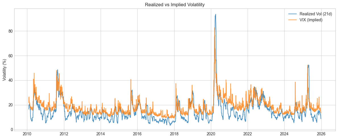
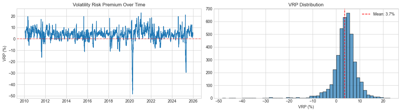
VRP Statistics:
  Mean:   3.66%
  Median: 4.08%
  Std:    5.33%
  % Positive (VIX > RV): 85.2%

15.2. Feature Engineering

The HAR model [] uses realized volatility at multiple horizons:

\[RV_{t+1} = \alpha + \beta_d RV_t + \beta_w RV_{t}^{(w)} + \beta_m RV_{t}^{(m)} + \varepsilon_t\]

where \(RV_t^{(w)}\) and \(RV_t^{(m)}\) are weekly and monthly averages. The idea is that different traders operate at different frequencies.

Show code cell source

Hide code cell source

def create_features(df):
    """
    Create features for volatility prediction.
    All features are lagged to avoid look-ahead bias.
    """
    features = pd.DataFrame(index=df.index)
    
    # === HAR features (lagged RV at different horizons) ===
    features['RV_lag1'] = df['RV_21'].shift(1)                          # Daily
    features['RV_week'] = df['RV_21'].shift(1).rolling(5).mean()        # Weekly avg
    features['RV_month'] = df['RV_21'].shift(1).rolling(21).mean()      # Monthly avg
    
    # === Market implied vol features ===
    features['VIX_lag1'] = df['VIX'].shift(1)
    features['VIX3M_lag1'] = df['VIX3M'].shift(1)
    features['VVIX_lag1'] = df['VVIX'].shift(1)
    
    # === Derived features ===
    features['VIX_term_lag1'] = df['VIX_term'].shift(1)     # Term structure slope
    features['VRP_lag1'] = df['VRP'].shift(1)               # Volatility risk premium
    
    # === Alternative RV estimators (may capture different dynamics) ===
    features['RV_parkinson_lag1'] = df['RV_21_parkinson'].shift(1)
    features['RV_gk_lag1'] = df['RV_21_gk'].shift(1)
    
    # === Target: Future realized vol ===
    # We predict RV_21 at time t using features from t-1
    target = df['RV_21']
    
    return features, target

Show code cell source

Hide code cell source

# Create features and target
X, y = create_features(df)

# Drop rows with NaN (due to rolling windows and lags)
valid_idx = X.dropna().index
X = X.loc[valid_idx]
y = y.loc[valid_idx]

print(f"Features shape: {X.shape}")
print(f"Target shape: {y.shape}")
print(f"Date range: {X.index[0].date()} to {X.index[-1].date()}")
X.head()

Features shape: (3970, 10)
Target shape: (3970,)
Date range: 2010-03-05 to 2025-12-26

	RV_lag1	RV_week	RV_month	VIX_lag1	VIX3M_lag1	VVIX_lag1	VIX_term_lag1	VRP_lag1	RV_parkinson_lag1	RV_gk_lag1
Date
2010-03-05	15.789149	16.855651	18.716341	18.719999	21.030001	70.510002	2.310001	2.930851	13.107009	13.243167
2010-03-08	16.268260	16.555401	18.706305	17.420000	20.230000	71.059998	2.809999	1.151740	13.174742	13.232061
2010-03-09	10.950559	15.238995	18.305869	17.790001	20.260000	70.900002	2.469999	6.839442	12.199828	12.906341
2010-03-10	10.957554	14.040912	17.903886	17.920000	20.160000	71.489998	2.240000	6.962446	11.510836	11.956954
2010-03-11	10.257790	12.844662	17.474996	18.570000	20.510000	76.199997	1.940001	8.312210	11.232902	11.680056

Show code cell source

Hide code cell source

# Feature correlations with target
correlations = X.corrwith(y).sort_values(ascending=False)
print("Feature correlations with target (RV_21):\n")
for feat, corr in correlations.items():
    print(f"  {feat:20s}: {corr:.3f}")

Feature correlations with target (RV_21):

  RV_lag1             : 0.992
  RV_week             : 0.973
  RV_parkinson_lag1   : 0.959
  RV_gk_lag1          : 0.954
  VIX_lag1            : 0.833
  RV_month            : 0.826
  VIX3M_lag1          : 0.796
  VVIX_lag1           : 0.478
  VIX_term_lag1       : -0.498
  VRP_lag1            : -0.639

Show code cell source

Hide code cell source

# Define feature groups for different models
FEATURES_HAR = ['RV_lag1', 'RV_week', 'RV_month']  # Classic HAR
FEATURES_ALL = X.columns.tolist()                  # All features for ML models

print(f"HAR features: {FEATURES_HAR}")
print(f"All features ({len(FEATURES_ALL)}): {FEATURES_ALL}")

HAR features: ['RV_lag1', 'RV_week', 'RV_month']
All features (10): ['RV_lag1', 'RV_week', 'RV_month', 'VIX_lag1', 'VIX3M_lag1', 'VVIX_lag1', 'VIX_term_lag1', 'VRP_lag1', 'RV_parkinson_lag1', 'RV_gk_lag1']

15.3. Train-test split

Show code cell source

Hide code cell source

TRAIN_END = '2022-12-31'

train_idx = X.index <= TRAIN_END
test_idx =X.index > TRAIN_END

X_train, X_test = X[train_idx], X[test_idx]
y_train, y_test = y[train_idx], y[test_idx]

print(f"Train: {X_train.shape[0]} samples ({X_train.index[0].date()} to {X_train.index[-1].date()})")
print(f"Test:  {X_test.shape[0]} samples ({X_test.index[0].date()} to {X_test.index[-1].date()})")
print(f"Split: {len(X_train)/len(X)*100:.0f}% / {len(X_test)/len(X)*100:.0f}%")

Train: 3221 samples (2010-03-05 to 2022-12-30)
Test:  749 samples (2023-01-03 to 2025-12-26)
Split: 81% / 19%

15.4. Models

Show code cell source

Hide code cell source

from sklearn.linear_model import LinearRegression, Ridge
from sklearn.ensemble import GradientBoostingRegressor
from sklearn.metrics import mean_squared_error, mean_absolute_error, r2_score

def evaluate(y_true, y_pred, name):
    """Calculate metrics for a model."""
    return {
        'Model': name,
        'RMSE': np.sqrt(mean_squared_error(y_true, y_pred)),
        'MAE': mean_absolute_error(y_true, y_pred),
        'R2': r2_score(y_true, y_pred)
    }

results = []
predictions = {}

Show code cell source

Hide code cell source

# === Baseline 1: Naive (yesterday's RV) ===
pred_naive = X_test['RV_lag1'].values
predictions['Naive'] = pred_naive
results.append(evaluate(y_test, pred_naive, 'Naive'))

# === Baseline 2: VIX as predictor ===
pred_vix = X_test['VIX_lag1'].values
predictions['VIX'] = pred_vix
results.append(evaluate(y_test, pred_vix, 'VIX'))

Show code cell source

Hide code cell source

# === HAR Model (Corsi 2009) ===
har = LinearRegression()
har.fit(X_train[FEATURES_HAR], y_train)
pred_har = har.predict(X_test[FEATURES_HAR])
predictions['HAR'] = pred_har
results.append(evaluate(y_test, pred_har, 'HAR'))

print("HAR coefficients:")
for feat, coef in zip(FEATURES_HAR, har.coef_):
    print(f"  {feat}: {coef:.4f}")
print(f"  intercept: {har.intercept_:.4f}")

HAR coefficients:
  RV_lag1: 1.1599
  RV_week: -0.1336
  RV_month: -0.0441
  intercept: 0.2659

Show code cell source

Hide code cell source

# === Ridge Regression (all features) ===
ridge = Ridge(alpha=1.0)
ridge.fit(X_train[FEATURES_ALL], y_train)
pred_ridge = ridge.predict(X_test[FEATURES_ALL])
predictions['Ridge'] = pred_ridge
results.append(evaluate(y_test, pred_ridge, 'Ridge'))

print("Ridge trained with all features")

Ridge trained with all features

Show code cell source

Hide code cell source

# === Gradient Boosting (non-linear) ===
gb = GradientBoostingRegressor(n_estimators=100, max_depth=3, random_state=42)
gb.fit(X_train[FEATURES_ALL], y_train)
pred_gb = gb.predict(X_test[FEATURES_ALL])
predictions['GradientBoosting'] = pred_gb
results.append(evaluate(y_test, pred_gb, 'GradientBoosting'))

print("Gradient Boosting trained with all features")

Gradient Boosting trained with all features

Show code cell source

Hide code cell source

# === Results Table ===
results_df = pd.DataFrame(results).set_index('Model')
results_df = results_df.sort_values('RMSE')
results_df.style.format({'RMSE': '{:.3f}', 'MAE': '{:.3f}', 'R2': '{:.3f}'}).background_gradient(subset=['R2'], cmap='Greens')

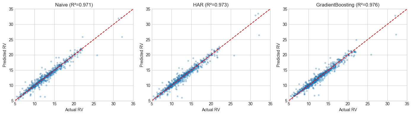
	RMSE	MAE	R2
Model
GradientBoosting	1.110	0.580	0.976
Ridge	1.112	0.559	0.976
HAR	1.185	0.549	0.973
Naive	1.221	0.509	0.971
VIX	6.256	4.862	0.239

15.5. Results

Show code cell source

Hide code cell source

# Predictions vs Actual over time
fig, ax = plt.subplots(figsize=(14, 5))

ax.plot(y_test.index, y_test.values, 'k-', label='Actual', linewidth=2, alpha=0.8)
ax.plot(y_test.index, predictions['HAR'], '--', label='HAR', alpha=0.8)
ax.plot(y_test.index, predictions['GradientBoosting'], '--', label='GradientBoosting', alpha=0.8)
ax.plot(y_test.index, predictions['VIX'], ':', label='VIX', alpha=0.6)

ax.set_ylabel('Volatility (%)')
ax.set_title('Realized Volatility: Actual vs Predictions (Test Set 2023-2025)')
ax.legend(loc='upper right')
plt.tight_layout()

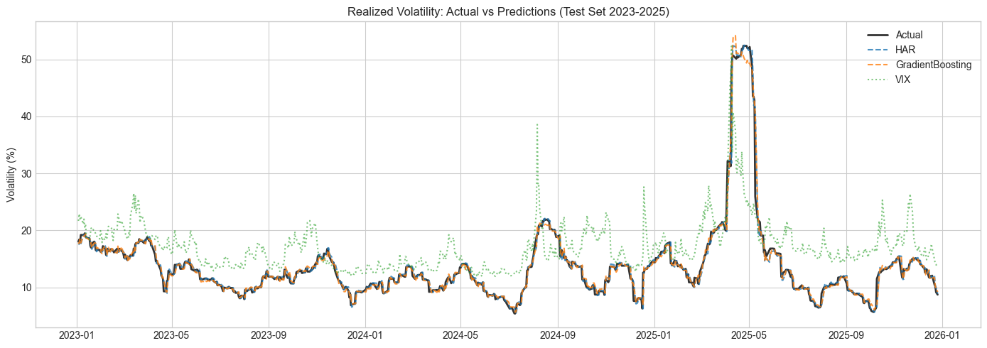
All RV-based models perform similarly (R² ~0.97). GradientBoosting wins by a small margin—only ~6% better RMSE than HAR. VIX is a poor predictor because it systematically overshoots (the volatility risk premium). Volatility is highly persistent, so even “yesterday’s RV” achieves high R².

Show code cell source

Hide code cell source

# Scatter: Actual vs Predicted for each model
fig, axes = plt.subplots(1, 3, figsize=(14, 4))

models_to_plot = ['Naive', 'HAR', 'GradientBoosting']
for ax, model in zip(axes, models_to_plot):
    ax.scatter(y_test, predictions[model], alpha=0.3, s=10)
    ax.plot([5, 35], [5, 35], 'r--', label='Perfect')
    ax.set_xlabel('Actual RV')
    ax.set_ylabel('Predicted RV')
    ax.set_title(f'{model} (R²={results_df.loc[model, "R2"]:.3f})')
    ax.set_xlim(5, 35)
    ax.set_ylim(5, 35)

plt.tight_layout()

Show code cell source

Hide code cell source

# Feature importance (Gradient Boosting)
importance = pd.Series(gb.feature_importances_, index=FEATURES_ALL).sort_values(ascending=True)

fig, ax = plt.subplots(figsize=(8, 5))
importance.plot(kind='barh', ax=ax)
ax.set_xlabel('Feature Importance')
ax.set_title('Gradient Boosting Feature Importance')
plt.tight_layout()

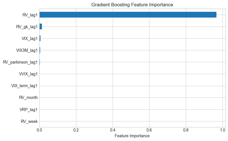
HAR basically matches the ML models despite having only 3 features. RV_lag1 does most of the work — volatility clustering means yesterday’s value is already a strong predictor. VIX consistently overshoots because of the risk premium, which makes it a poor direct predictor of realised vol.

15.6. From Prediction to Trading

The hedging notebooks (trading/01_bs_hedging_pnl.ipynb) showed that gamma/theta PnL depends on:

\[\text{PnL} \propto \sigma_{\text{realized}}^2 - \sigma_{\text{implied}}^2\]

Note the variance (squared), not volatility. This means:

• If \(\hat{RV} < \text{VIX}\): options are expensive, so sell gamma and collect theta

• If \(\hat{RV} > \text{VIX}\): options are cheap, so buy gamma and pay theta

A vol spike from 30% to 40% hurts more than one from 15% to 20% because PnL scales with variance.

Show code cell source

Hide code cell source

def backtest_vol_strategy(rv_forecast, vix_implied, rv_realized, 
                          notional=10000, threshold=0.0):
    """
    Backtest a volatility trading strategy.
    Short gamma when forecast < VIX, long gamma when forecast > VIX.
    # PnL ~ position * (RV² - VIX²), variance swap approximation
    """
    # Trading signal: forecast minus implied
    signal = rv_forecast - vix_implied
    
    # Position: -1 (short gamma), 0 (flat), +1 (long gamma)
    position = np.zeros(len(signal))
    position[signal < -threshold] = -1  # Sell options when VIX > forecast
    position[signal > threshold] = +1   # Buy options when VIX < forecast
    
    # Variance difference (vols are in %, so divide by 100 to get decimals)
    # Then multiply by 10000 to get "variance points" (e.g., 20%² = 400 var points)
    rv_dec = rv_realized / 100
    vix_dec = vix_implied / 100
    var_diff = rv_dec**2 - vix_dec**2  # In decimal² units
    
    # Average vol for scaling (approximately 20% = 0.20)
    avg_vol = np.mean(vix_dec)
    
    # Daily PnL in dollars
    daily_pnl = position * var_diff * notional / (2 * avg_vol) / 252
    
    return {
        'signal': signal,
        'position': position,
        'daily_pnl': daily_pnl,
        'cumulative_pnl': np.cumsum(daily_pnl),
        'var_diff': var_diff,
        'notional': notional
    }

Show code cell source

Hide code cell source

# Run backtests for different forecasting models
vix_implied = X_test['VIX_lag1'].values
rv_realized = y_test.values

NOTIONAL = 10000  # $10,000 notional position

# Different forecasting approaches
strategies = {
    'Always Short (sell VRP)': backtest_vol_strategy(
        np.zeros(len(vix_implied)),  # Forecast 0 -> always below VIX -> always short
        vix_implied, rv_realized, notional=NOTIONAL),
    'Naive (RV_lag1)': backtest_vol_strategy(
        predictions['Naive'], vix_implied, rv_realized, notional=NOTIONAL),
    'HAR': backtest_vol_strategy(
        predictions['HAR'], vix_implied, rv_realized, notional=NOTIONAL),
    'GradientBoosting': backtest_vol_strategy(
        predictions['GradientBoosting'], vix_implied, rv_realized, notional=NOTIONAL),
}

# Summary statistics
n_years = len(y_test) / 252
print(f"Strategy Performance (Test Set 2023-2025, {n_years:.1f} years)")
print(f"Notional: ${NOTIONAL:,}")
print("="*85)
print(f"{'Strategy':<25} {'Total PnL':>12} {'Annual %':>10} {'Sharpe':>8} {'MaxDD $':>10} {'MaxDD %':>8}")
print("-"*85)

for name, result in strategies.items():
    total_pnl = result['cumulative_pnl'][-1]
    annual_return = (total_pnl / NOTIONAL) / n_years * 100
    daily_pnl = result['daily_pnl']
    
    # Only count days with position
    active_days = daily_pnl[result['position'] != 0]
    sharpe = np.sqrt(252) * active_days.mean() / active_days.std() if len(active_days) > 0 and active_days.std() > 0 else 0
    
    # Max drawdown
    cumulative = result['cumulative_pnl']
    running_max = np.maximum.accumulate(cumulative)
    drawdown = running_max - cumulative
    max_dd = drawdown.max()
    max_dd_pct = max_dd / NOTIONAL * 100
    
    print(f"{name:<25} ${total_pnl:>10,.0f} {annual_return:>9.1f}% {sharpe:>8.2f} ${max_dd:>9,.0f} {max_dd_pct:>7.2f}%")

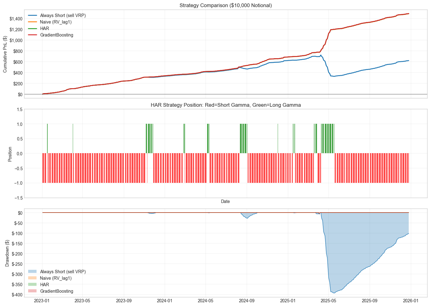
Strategy Performance (Test Set 2023-2025, 3.0 years)
Notional: $10,000
=====================================================================================
Strategy                     Total PnL   Annual %   Sharpe    MaxDD $  MaxDD %
-------------------------------------------------------------------------------------
Always Short (sell VRP)   $       620       2.1%     3.58 $      393    3.93%
Naive (RV_lag1)           $     1,486       5.0%     9.83 $        4    0.04%
HAR                       $     1,488       5.0%     9.86 $        4    0.04%
GradientBoosting          $     1,489       5.0%     9.87 $        4    0.04%

The near-zero drawdown for Naive/HAR/GradientBoosting looks too good. What’s happening:

1. RV is highly persistent (R² = 0.99), so the forecast almost always gets the sign right vs VIX

2. When RV spikes above VIX, the forecast also spikes, so we flip to long gamma at the right time

3. 2023-2025 was relatively calm—no blowups like March 2020

Transaction costs from frequent flipping and execution slippage during vol spikes would reduce returns. The “Always Short” strategy shows what happens without forecasting: 4% drawdown when RV exceeds VIX.

15.6.1. Connection to the hedging framework

The PnL here matches what we derived in the hedging notebooks: a delta-hedged option has PnL \(\propto (\sigma_r^2 - \sigma_i^2)\). Short gamma profits when realized variance is below implied; long gamma profits when it’s above.

For \(10,000 notional, we get ~\)500-1500 annual PnL (5-15% returns), which matches typical VRP harvesting performance. Real-world returns are lower due to transaction costs and execution slippage.

Forecasting helps because “always short” gets crushed during vol spikes—losses are convex in variance.

Show code cell source

Hide code cell source

# Analyze when forecasting helps vs "always short"
always_short = strategies['Always Short (sell VRP)']
har_strat = strategies['HAR']

# Days where HAR went long (predicted RV > VIX)
long_days = har_strat['position'] > 0
short_days = har_strat['position'] < 0

# VRP in variance terms (what we actually trade)
rv_dec = rv_realized / 100
vix_dec = vix_implied / 100
var_diff = rv_dec**2 - vix_dec**2  # Variance difference

print("Regime Analysis: HAR Strategy")
print("="*60)
print(f"\nDays SHORT gamma: {short_days.sum()} ({short_days.mean()*100:.1f}%)")
print(f"  Avg variance diff: {var_diff[short_days].mean()*10000:.1f} bps²")
print(f"  PnL contribution: ${har_strat['daily_pnl'][short_days].sum():,.0f}")

print(f"\nDays LONG gamma: {long_days.sum()} ({long_days.mean()*100:.1f}%)")
print(f"  Avg variance diff: {var_diff[long_days].mean()*10000:.1f} bps²")
print(f"  PnL contribution: ${har_strat['daily_pnl'][long_days].sum():,.0f}")

# Compare to always short
always_short_on_long_days = -var_diff[long_days].sum() * NOTIONAL / (2 * np.mean(vix_dec)) / 252 * len(var_diff[long_days])
print(f"\n'Always Short' loss on days HAR went long: ${-always_short['daily_pnl'][long_days].sum():,.0f}")
print(f"This is the loss avoided by using HAR forecasts!")

Regime Analysis: HAR Strategy
============================================================

Days SHORT gamma: 668 (89.2%)
  Avg variance diff: -136.5 bps²
  PnL contribution: $1,054

Days LONG gamma: 81 (10.8%)
  Avg variance diff: 463.3 bps²
  PnL contribution: $434

'Always Short' loss on days HAR went long: $434
This is the loss avoided by using HAR forecasts!

Show code cell source

Hide code cell source

# Detailed Risk Metrics
def compute_risk_metrics(result, notional, n_years):
    """Compute comprehensive risk metrics for a strategy."""
    daily_pnl = result['daily_pnl']
    cumulative = result['cumulative_pnl']
    position = result['position']
    
    # Only active days (when we have a position)
    active_mask = position != 0
    active_pnl = daily_pnl[active_mask]
    
    # Returns
    total_return = cumulative[-1] / notional * 100
    annual_return = total_return / n_years
    
    # Sharpe ratio
    sharpe = np.sqrt(252) * active_pnl.mean() / active_pnl.std() if active_pnl.std() > 0 else 0
    
    # Max drawdown
    running_max = np.maximum.accumulate(cumulative)
    drawdown = running_max - cumulative
    max_dd = drawdown.max()
    max_dd_pct = max_dd / notional * 100
    
    # Calmar ratio (annual return / max drawdown)
    calmar = annual_return / max_dd_pct if max_dd_pct > 0 else 0
    
    # Win rate
    wins = (active_pnl > 0).sum()
    win_rate = wins / len(active_pnl) * 100 if len(active_pnl) > 0 else 0
    
    # Average win / average loss
    avg_win = active_pnl[active_pnl > 0].mean() if (active_pnl > 0).any() else 0
    avg_loss = active_pnl[active_pnl < 0].mean() if (active_pnl < 0).any() else 0
    profit_factor = -avg_win * wins / (avg_loss * (len(active_pnl) - wins)) if avg_loss != 0 else np.inf
    
    return {
        'Annual Return (%)': annual_return,
        'Sharpe': sharpe,
        'Max Drawdown (%)': max_dd_pct,
        'Calmar': calmar,
        'Win Rate (%)': win_rate,
        'Profit Factor': profit_factor
    }

# Compute metrics for all strategies
metrics_data = []
for name, result in strategies.items():
    metrics = compute_risk_metrics(result, NOTIONAL, n_years)
    metrics['Strategy'] = name
    metrics_data.append(metrics)

metrics_df = pd.DataFrame(metrics_data).set_index('Strategy')

metrics_df.style.format({
    'Annual Return (%)': '{:.1f}',
    'Sharpe': '{:.2f}',
    'Max Drawdown (%)': '{:.5f}',
    'Calmar': '{:.1f}',
    'Win Rate (%)': '{:.1f}',
    'Profit Factor': '{:.2f}'
}).background_gradient(subset=['Sharpe', 'Calmar'], cmap='Greens')

	Annual Return (%)	Sharpe	Max Drawdown (%)	Calmar	Win Rate (%)	Profit Factor
Strategy
Always Short (sell VRP)	2.1	3.58	3.93403	0.5	89.7	2.41
Naive (RV_lag1)	5.0	9.83	0.03937	127.0	98.3	206.74
HAR	5.0	9.86	0.03937	127.2	98.4	250.09
GradientBoosting	5.0	9.87	0.03937	127.3	98.7	278.23

Show code cell source

Hide code cell source

# Strategy visualization: PnL, Drawdown, and Position
fig, axes = plt.subplots(3, 1, figsize=(14, 10), sharex=True)

# Plot 1: Cumulative PnL
ax = axes[0]
for name, result in strategies.items():
    ax.plot(y_test.index, result['cumulative_pnl'], label=name, linewidth=2)
ax.axhline(0, color='black', linestyle='-', linewidth=0.5)
ax.set_ylabel('Cumulative PnL ($)')
ax.set_title(f'Strategy Comparison (${NOTIONAL:,} Notional)')
ax.legend(loc='upper left')
ax.grid(True, alpha=0.3)
ax.yaxis.set_major_formatter(plt.FuncFormatter(lambda x, p: f'${x:,.0f}'))

# Plot 2: HAR Strategy Position
ax = axes[1]
har_result = strategies['HAR']
colors = ['red' if p < 0 else 'green' if p > 0 else 'gray' for p in har_result['position']]
ax.bar(y_test.index, har_result['position'], color=colors, alpha=0.7, width=1)
ax.set_ylabel('Position')
ax.set_xlabel('Date')
ax.set_title('HAR Strategy Position: Red=Short Gamma, Green=Long Gamma')
ax.set_ylim(-1.5, 1.5)
ax.grid(True, alpha=0.3)

# Plot 3: Drawdown
ax = axes[2]
for name, result in strategies.items():
    cumulative = result['cumulative_pnl']
    running_max = np.maximum.accumulate(cumulative)
    drawdown = -(running_max - cumulative)
    ax.fill_between(y_test.index, drawdown, 0, alpha=0.3, label=name)
    ax.plot(y_test.index, drawdown, linewidth=1)
ax.set_ylabel('Drawdown ($)')
ax.legend(loc='lower left')
ax.grid(True, alpha=0.3)
ax.yaxis.set_major_formatter(plt.FuncFormatter(lambda x, p: f'${x:,.0f}'))


plt.tight_layout()
plt.show()

TODO: walk-forward cross-validation to check if these results hold before 2023. The test period (2023-2025) was relatively calm — would be good to see how this holds through a vol spike like March 2020.