3. Heston Calibration

Can we recover Heston [1993] parameters from option prices? We generate synthetic market data from known parameters, calibrate back, and see what breaks.

SLSQP with a single starting point gets kappa wrong by 35% — the loss surface is flat in that direction. Levenberg-Marquardt does better, and the Hessian eigenspectrum shows exactly why.

Show code cell source

Hide code cell source

import numpy as np
import matplotlib.pyplot as plt
plt.style.use('ggplot')
from scipy.optimize import minimize, least_squares, differential_evolution
import warnings
import time

import sys
sys.path.insert(0, '..')
from utils import Heston_CF, Heston_price, bs_call_price, bs_vega, implied_vol, cos_price

import cppfm

3.1. COS Pricing

COS [Fang and Oosterlee, 2008] encodes the payoff directly in Fourier-cosine coefficients — no numerical integration, exponential convergence. The characteristic function uses the stable formulation from Albrecher et al. [2007] to avoid the branch cut issue.

Show code cell source

Hide code cell source

def Heston_price_COS(S0, K, T, r, kappa, nu0, theta, xi, rho, N=128):
    """Heston call price via COS method. """
    # CF of log-returns: phi(u) for ln(S_T/S_0)
    # Heston_CF gives E[exp(iu*ln(S_T))], so divide by S0^{iu}
    def cf(u):
        return Heston_CF(u, S0, T, r, kappa, nu0, theta, xi, rho) / S0**(1j*u)

    # time-averaged variance for domain truncation
    # E[∫v_s ds] / T ≈ (ν₀ - θ)(1 - e^{-κT})/(κT) + θ
    if abs(kappa * T) > 1e-8:
        avg_var = (nu0 - theta) / (kappa * T) * (1 - np.exp(-kappa * T)) + theta
    else:
        avg_var = nu0  # small T limit
    std = np.sqrt(max(avg_var, 1e-6))

    return cos_price(S0, K, T, r, cf, N=N, L=10, opt_type='call', std=std)

3.2. Sanity check: COS convergence

Gil-Pelaez with n=200 is itself approximate. We use a high-resolution reference (n=10000) and check both methods against it.

Show code cell source

Hide code cell source

# test params
S0 = 100
r = 0.05
kappa, nu0, theta, xi, rho = 0.8, 0.3**2, 0.3**2, 0.5, -0.8

test_cases = [
    (80, 0.25),
    (100, 0.5),
    (120, 1.0),
    (90, 0.25),
    (110, 0.5),
]

print(f"{'K':>6} {'T':>6} {'Reference':>12} {'COS(128)':>12} {'GP(200)':>12} {'COS err':>10} {'GP err':>10}")
print("-" * 75)

for K, T in test_cases:
    price_ref = Heston_price(S0, K, T, r, kappa, nu0, theta, xi, rho, n=10000, umax=200)
    price_cos = Heston_price_COS(S0, K, T, r, kappa, nu0, theta, xi, rho)
    price_gp = Heston_price(S0, K, T, r, kappa, nu0, theta, xi, rho)
    err_cos = abs(price_cos - price_ref)
    err_gp = abs(price_gp - price_ref)
    print(f"{K:>6.0f} {T:>6.2f} {price_ref:>12.6f} {price_cos:>12.6f} {price_gp:>12.6f} {err_cos:>10.2e} {err_gp:>10.2e}")

     K      T    Reference     COS(128)      GP(200)    COS err     GP err
---------------------------------------------------------------------------

    80   0.25    21.673670    21.673670    21.672486   4.26e-10   1.18e-03

   100   0.50     9.323819     9.323819     9.324225   3.78e-08   4.06e-04

   120   1.00     4.396658     4.396657     4.396639   2.85e-07   1.85e-05

    90   0.25    13.211971    13.211971    13.210964   5.23e-10   1.01e-03

   110   0.50     4.452662     4.452662     4.452337   2.00e-08   3.26e-04

3.3. Synthetic market data

We know the true parameters, so we can measure how badly calibration recovers them. Using COS for both data generation and calibration — otherwise method mismatch contaminates the experiment.

Show code cell source

Hide code cell source

# "true" Heston parameters (what we want to recover)
r = 0.05
S0 = 100
true_kappa = 1.5
true_nu0 = 0.04      # vol = 20%
true_theta = 0.06    # vol = 24.5%
true_xi = 0.4
true_rho = -0.7
true_params = [true_kappa, true_nu0, true_theta, true_xi, true_rho]

# wider strike range: ±20% moneyness gives the optimizer skew + curvature info
K_strikes = [80, 85, 90, 95, 100, 105, 110, 115, 120]
T_maturities = [0.25, 0.5, 1.0]

K_mkt = K_strikes * len(T_maturities)
T_mkt = sum([[T]*len(K_strikes) for T in T_maturities], [])
n_instruments = len(K_mkt)

# generate with COS — same method we'll calibrate with
Price_mkt = [Heston_price_COS(S0, K_mkt[i], T_mkt[i], r, *true_params) for i in range(n_instruments)]
IV_mkt = [implied_vol(Price_mkt[i], S0, K_mkt[i], r, T_mkt[i]) for i in range(n_instruments)]

print(f"True params: kappa={true_kappa}, nu0={true_nu0:.4f}, theta={true_theta:.4f}, xi={true_xi}, rho={true_rho}")
print(f"Feller check: 2*kappa*theta - xi^2 = {2*true_kappa*true_theta - true_xi**2:.4f} > 0")
print(f"{n_instruments} instruments across {len(T_maturities)} maturities, strikes {K_strikes[0]}-{K_strikes[-1]}\n")

print(f"{'K':>8} {'T':>6} {'IV':>8} {'Price':>10}")
for i in range(n_instruments):
    print(f"{K_mkt[i]:>8.1f} {T_mkt[i]:>6.2f} {IV_mkt[i]:>8.1%} {Price_mkt[i]:>10.4f}")

True params: kappa=1.5, nu0=0.0400, theta=0.0600, xi=0.4, rho=-0.7
Feller check: 2*kappa*theta - xi^2 = 0.0200 > 0
27 instruments across 3 maturities, strikes 80-120

       K      T       IV      Price
    80.0   0.25    26.3%    21.1631
    85.0   0.25    24.9%    16.4659
    90.0   0.25    23.4%    12.0261
    95.0   0.25    22.0%     8.0282
   100.0   0.25    20.5%     4.7065
   105.0   0.25    19.0%     2.2859
   110.0   0.25    17.6%     0.8577
   115.0   0.25    16.6%     0.2398
   120.0   0.25    16.0%     0.0524
    80.0   0.50    26.0%    22.6400
    85.0   0.50    24.7%    18.2513
    90.0   0.50    23.5%    14.1344
    95.0   0.50    22.2%    10.3915
   100.0   0.50    20.9%     7.1382
   105.0   0.50    19.7%     4.4886
   110.0   0.50    18.5%     2.5250
   115.0   0.50    17.5%     1.2485
   120.0   0.50    16.7%     0.5434
    80.0   1.00    25.7%    25.5434
    85.0   1.00    24.6%    21.5169
    90.0   1.00    23.6%    17.7304
    95.0   1.00    22.6%    14.2345
   100.0   1.00    21.7%    11.0814
   105.0   1.00    20.8%     8.3204
   110.0   1.00    19.9%     5.9915
   115.0   1.00    19.1%     4.1158
   120.0   1.00    18.3%     2.6871

3.4. Calibration setup

Two objectives: MSE on prices vs MSE on implied vols. Feller constraint \(2\kappa\theta > \xi^2\) enforced via both inequality constraints and explicit parameter bounds.

Show code cell source

Hide code cell source

# params = [kappa, nu0, theta, xi, rho]
param_names = ['kappa', 'nu0', 'theta', 'xi', 'rho']

def MSE_Price_COS(params):
    """MSE between market and model prices using COS."""
    mse = 0
    for i in range(n_instruments):
        model_price = Heston_price_COS(S0, K_mkt[i], T_mkt[i], r, *params)
        mse += (model_price - Price_mkt[i])**2
    return mse / n_instruments

def MSE_IV_COS(params):
    """MSE between market and model implied vols using COS."""
    mse = 0
    for i in range(n_instruments):
        model_price = Heston_price_COS(S0, K_mkt[i], T_mkt[i], r, *params)
        model_iv = implied_vol(model_price, S0, K_mkt[i], r, T_mkt[i])
        mse += (model_iv - IV_mkt[i])**2
    return mse / n_instruments

def residuals_price_COS(params):
    """Residual vector for least_squares (price differences)."""
    res = np.zeros(n_instruments)
    for i in range(n_instruments):
        res[i] = Heston_price_COS(S0, K_mkt[i], T_mkt[i], r, *params) - Price_mkt[i]
    return res

def residuals_iv_COS(params):
    """Residual vector for least_squares (IV differences)."""
    res = np.zeros(n_instruments)
    for i in range(n_instruments):
        model_price = Heston_price_COS(S0, K_mkt[i], T_mkt[i], r, *params)
        res[i] = implied_vol(model_price, S0, K_mkt[i], r, T_mkt[i]) - IV_mkt[i]
    return res

# explicit bounds: [kappa, nu0, theta, xi, rho]
bounds_lower = [0.01, 1e-4, 1e-4, 0.01, -0.999]
bounds_upper = [20.0, 1.0, 1.0, 3.0, 0.999]

# SLSQP constraints (redundant with bounds, but SLSQP uses these)
cons = (
    {'type': 'ineq', 'fun': lambda x: x[0] - bounds_lower[0]},
    {'type': 'ineq', 'fun': lambda x: bounds_upper[0] - x[0]},
    {'type': 'ineq', 'fun': lambda x: x[1] - bounds_lower[1]},
    {'type': 'ineq', 'fun': lambda x: x[2] - bounds_lower[2]},
    {'type': 'ineq', 'fun': lambda x: x[3] - bounds_lower[3]},
    {'type': 'ineq', 'fun': lambda x: bounds_upper[4] - abs(x[4])},
    # Feller: 2*kappa*theta > xi^2 (no artificial buffer)
    {'type': 'ineq', 'fun': lambda x: 2 * x[0] * x[2] - x[3]**2}
)

def print_calib_result(params_calib, result_obj=None):
    """Print calibration results with convergence info."""
    print(f"{'Param':>8} {'Calibrated':>12} {'True':>12} {'Rel Error':>12}")
    print("-" * 48)
    for i, name in enumerate(param_names):
        calib = params_calib[i]
        true = true_params[i]
        rel_err = abs(calib - true) / abs(true) if abs(true) > 1e-10 else abs(calib - true)
        print(f"{name:>8} {calib:>12.6f} {true:>12.4f} {rel_err:>11.2%}")
    feller = 2*params_calib[0]*params_calib[2] - params_calib[3]**2
    print(f"\nFeller: 2*kappa*theta - xi^2 = {feller:.4f} {'> 0' if feller > 0 else '< 0 VIOLATED'}")
    if result_obj is not None and hasattr(result_obj, 'success'):
        print(f"Converged: {result_obj.success}, Iterations: {result_obj.nit}, Final MSE: {result_obj.fun:.2e}")

3.5. Price-MSE calibration

Show code cell source

Hide code cell source

warnings.filterwarnings('ignore', category=RuntimeWarning)

# initial params: [kappa, nu0, theta, xi, rho]
params0 = [2.0, 0.25**2, 0.25**2, 0.5, -0.8]

t0 = time.time()
result_price_cos = minimize(MSE_Price_COS, params0, constraints=cons, method='SLSQP',
                            bounds=list(zip(bounds_lower, bounds_upper)), tol=1e-8)
time_price_cos = time.time() - t0

params_price_cos = result_price_cos['x']
print(f"SLSQP Price-MSE calibration ({time_price_cos:.2f}s)\n")
print_calib_result(params_price_cos, result_price_cos)

SLSQP Price-MSE calibration (0.94s)

   Param   Calibrated         True    Rel Error
------------------------------------------------
   kappa     1.500004       1.5000       0.00%
     nu0     0.040000       0.0400       0.00%
   theta     0.059998       0.0600       0.00%
      xi     0.399911       0.4000       0.02%
     rho    -0.700125      -0.7000       0.02%

Feller: 2*kappa*theta - xi^2 = 0.0201 > 0
Converged: True, Iterations: 25, Final MSE: 9.84e-10

3.6. IV-MSE calibration

Does matching implied vols instead of prices help?

Show code cell source

Hide code cell source

params0 = [2.0, 0.25**2, 0.25**2, 0.5, -0.8]

t0 = time.time()
result_iv_cos = minimize(MSE_IV_COS, params0, constraints=cons, method='SLSQP',
                         bounds=list(zip(bounds_lower, bounds_upper)), tol=1e-10)
time_iv_cos = time.time() - t0

params_iv_cos = result_iv_cos['x']
print(f"SLSQP IV-MSE calibration ({time_iv_cos:.2f}s)\n")
print_calib_result(params_iv_cos, result_iv_cos)

SLSQP IV-MSE calibration (4.85s)

   Param   Calibrated         True    Rel Error
------------------------------------------------
   kappa     1.999940       1.5000      33.33%
     nu0     0.039804       0.0400       0.49%
   theta     0.056586       0.0600       5.69%
      xi     0.432592       0.4000       8.15%
     rho    -0.696388      -0.7000       0.52%

Feller: 2*kappa*theta - xi^2 = 0.0392 > 0
Converged: True, Iterations: 23, Final MSE: 7.15e-07

3.7. IV smile fit

Show code cell source

Hide code cell source

# model IVs for both SLSQP calibrations
IV_price_cos = [implied_vol(Heston_price_COS(S0, K_mkt[i], T_mkt[i], r, *params_price_cos), 
                            S0, K_mkt[i], r, T_mkt[i]) for i in range(n_instruments)]
IV_iv_cos = [implied_vol(Heston_price_COS(S0, K_mkt[i], T_mkt[i], r, *params_iv_cos), 
                         S0, K_mkt[i], r, T_mkt[i]) for i in range(n_instruments)]

n_K = len(K_strikes)
fig, axs = plt.subplots(1, 3, figsize=(14, 4), sharey=True)

for j, T in enumerate(T_maturities):
    idx = slice(j*n_K, (j+1)*n_K)
    
    axs[j].scatter(K_strikes, IV_mkt[idx], s=80, c='black', marker='o', 
                   label='Market', zorder=3)
    axs[j].plot(K_strikes, IV_price_cos[idx], 'b-', lw=2, marker='s', 
                markersize=5, label='Price calib')
    axs[j].plot(K_strikes, IV_iv_cos[idx], 'r--', lw=2, marker='^', 
                markersize=5, label='IV calib')
    
    axs[j].set_xlabel('Strike')
    axs[j].set_title(f'T = {T}')
    axs[j].grid(True, alpha=0.3)

axs[0].set_ylabel('Implied Vol')
axs[0].legend(loc='upper right')
plt.suptitle('SLSQP calibrations vs Market', y=1.02)
plt.tight_layout()
plt.show()

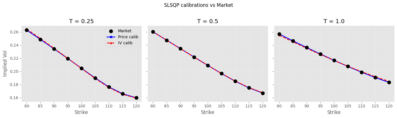
3.8. Python Levenberg-Marquardt

SLSQP treats the MSE as a scalar — it can’t see the structure of individual residuals. least_squares with method='trf' (trust-region reflective, LM variant with bounds support) exploits the least-squares structure and uses the Jacobian of the residual vector. Same Python, same COS pricer — only the algorithm changes.

Show code cell source

Hide code cell source

params0 = [2.0, 0.25**2, 0.25**2, 0.5, -0.8]

# price residuals
t0 = time.time()
result_lm_price = least_squares(residuals_price_COS, params0,
                                bounds=(bounds_lower, bounds_upper), method='trf')
time_lm_price = time.time() - t0
params_lm_price = result_lm_price.x

print(f"Python LM Price-MSE ({time_lm_price:.2f}s, {result_lm_price.nfev} func evals)\n")
print_calib_result(params_lm_price)

# IV residuals
t0 = time.time()
result_lm_iv = least_squares(residuals_iv_COS, params0,
                             bounds=(bounds_lower, bounds_upper), method='trf')
time_lm_iv = time.time() - t0
params_lm_iv = result_lm_iv.x

print(f"\nPython LM IV-MSE ({time_lm_iv:.2f}s, {result_lm_iv.nfev} func evals)\n")
print_calib_result(params_lm_iv)

Python LM Price-MSE (0.37s, 11 func evals)

   Param   Calibrated         True    Rel Error
------------------------------------------------
   kappa     1.500000       1.5000       0.00%
     nu0     0.040000       0.0400       0.00%
   theta     0.060000       0.0600       0.00%
      xi     0.400000       0.4000       0.00%
     rho    -0.700000      -0.7000       0.00%

Feller: 2*kappa*theta - xi^2 = 0.0200 > 0

Python LM IV-MSE (1.54s, 7 func evals)

   Param   Calibrated         True    Rel Error
------------------------------------------------
   kappa     1.500000       1.5000       0.00%
     nu0     0.040000       0.0400       0.00%
   theta     0.060000       0.0600       0.00%
      xi     0.400000       0.4000       0.00%
     rho    -0.700000      -0.7000       0.00%

Feller: 2*kappa*theta - xi^2 = 0.0200 > 0

3.9. Multi-start and global optimization

Single starting point on a flat loss surface is unreliable. differential_evolution searches globally — no starting point needed. We also run a multi-start SLSQP for comparison.

# differential evolution — global optimizer, no starting point bias
de_bounds = list(zip(bounds_lower, bounds_upper))

t0 = time.time()
result_de = differential_evolution(MSE_IV_COS, de_bounds, seed=42, tol=1e-8,
                                   maxiter=100, polish=True)
time_de = time.time() - t0
params_de = result_de.x

print(f"Differential Evolution IV-MSE ({time_de:.1f}s)\n")
print_calib_result(params_de, result_de)

# multi-start SLSQP: 20 random starting points, keep best
np.random.seed(42)
best_mse = np.inf
best_params = None
n_starts = 20

t0 = time.time()
for _ in range(n_starts):
    p0 = [np.random.uniform(lo, hi) for lo, hi in de_bounds]
    try:
        res = minimize(MSE_IV_COS, p0, constraints=cons, method='SLSQP',
                       bounds=de_bounds, tol=1e-10)
        if res.fun < best_mse:
            best_mse = res.fun
            best_params = res.x.copy()
    except:
        continue
time_ms = time.time() - t0

print(f"\nMulti-start SLSQP ({n_starts} starts, {time_ms:.1f}s)\n")
print_calib_result(best_params)

Differential Evolution IV-MSE (251.0s)

   Param   Calibrated         True    Rel Error
------------------------------------------------
   kappa     1.501055       1.5000       0.07%
     nu0     0.040000       0.0400       0.00%
   theta     0.059990       0.0600       0.02%
      xi     0.400074       0.4000       0.02%
     rho    -0.699965      -0.7000       0.01%

Feller: 2*kappa*theta - xi^2 = 0.0200 > 0
Converged: False, Iterations: 100, Final MSE: 4.95e-12

Multi-start SLSQP (20 starts, 127.4s)

   Param   Calibrated         True    Rel Error
------------------------------------------------
   kappa     1.501218       1.5000       0.08%
     nu0     0.040000       0.0400       0.00%
   theta     0.059995       0.0600       0.01%
      xi     0.400069       0.4000       0.02%
     rho    -0.700029      -0.7000       0.00%

Feller: 2*kappa*theta - xi^2 = 0.0201 > 0

# C++ Levenberg-Marquardt
# generate reference IVs from C++ pricer — same method for generation and calibration
# NOTE: C++ pricer uses a different pricing method (Gauss-Laguerre) than COS above,
# so the reference IVs differ by a few bps. The comparison chart is not perfectly
# apples-to-apples vs the Python calibrations, but the conclusion holds.

T_unique = T_maturities
K_unique = K_strikes
n_K = len(K_unique)

IV_mkt_cpp = []
for i in range(n_instruments):
    price_cpp = cppfm.heston_call_price(S0, K_mkt[i], r, T_mkt[i],
                                            true_kappa, true_theta, true_xi, true_rho, true_nu0)
    IV_mkt_cpp.append(cppfm.bs_implied_volatility(S0, K_mkt[i], r, T_mkt[i], price_cpp,
                                                    cppfm.OptionType.Call))

slices = []
for T in T_unique:
    s = cppfm.HestonSliceData()
    s.T = T
    mask = [i for i in range(n_instruments) if T_mkt[i] == T]
    s.strikes = [K_mkt[i] for i in mask]
    s.market_ivs = [IV_mkt_cpp[i] for i in mask]
    slices.append(s)

guess = cppfm.HestonParams(v0=0.25**2, kappa=2.0, vbar=0.25**2, sigma_v=0.5, rho=-0.8)

t0 = time.time()
result_cpp = cppfm.calibrate_heston(slices, S0=S0, r=r, guess=guess)
time_cpp = time.time() - t0

p = result_cpp.params
params_cpp = [p.kappa, p.v0, p.vbar, p.sigma_v, p.rho]
print(f"C++ LM: {result_cpp.iterations} iters, RMSE={result_cpp.rmse:.2e}, {time_cpp:.4f}s")
print(f"Converged: {result_cpp.converged}\n")
print_calib_result(params_cpp)

C++ LM: 6 iters, RMSE=4.86e-09, 0.0391s
Converged: True

   Param   Calibrated         True    Rel Error
------------------------------------------------
   kappa     1.499997       1.5000       0.00%
     nu0     0.040000       0.0400       0.00%
   theta     0.060000       0.0600       0.00%
      xi     0.400000       0.4000       0.00%
     rho    -0.700000      -0.7000       0.00%

Feller: 2*kappa*theta - xi^2 = 0.0200 > 0

# all-methods comparison
all_methods = {
    'SLSQP (1 start)': (params_iv_cos, time_iv_cos),
    'SLSQP (20 starts)': (best_params, time_ms),
    'Python LM (trf)': (params_lm_iv, time_lm_iv),
    'Diff. Evolution': (params_de, time_de),
    'C++ LM': (params_cpp, time_cpp),
}

n_methods = len(all_methods)
fig, (ax1, ax2) = plt.subplots(1, 2, figsize=(14, 5))

x = np.arange(5)
width = 0.15
colors = ['#d62728', '#ff7f0e', '#1f77b4', '#9467bd', '#2ca02c']

for j, (method, (params, _)) in enumerate(all_methods.items()):
    errors = [abs(params[i] - true_params[i]) / abs(true_params[i]) * 100 for i in range(5)]
    ax1.bar(x + (j - n_methods//2)*width, errors, width, label=method, color=colors[j])

ax1.set_xticks(x)
ax1.set_xticklabels([r'$\kappa$', r'$\nu_0$', r'$\theta$', r'$\xi$', r'$\rho$'], fontsize=12)
ax1.set_ylabel('Relative Error (%)')
ax1.set_title('Parameter Recovery (IV objective)')
ax1.legend(fontsize=8)
ax1.grid(True, alpha=0.3, axis='y')

# timing
method_names = list(all_methods.keys())
times_list = [t for _, t in all_methods.values()]
bars = ax2.bar(method_names, times_list, color=colors[:n_methods], edgecolor='black', linewidth=0.5)
ax2.set_ylabel('Time (s)')
ax2.set_title('Calibration Time')
for bar, t in zip(bars, times_list):
    label = f'{t:.2f}s' if t >= 0.1 else f'{t:.3f}s'
    ax2.text(bar.get_x() + bar.get_width()/2, bar.get_height() + max(times_list)*0.02,
             label, ha='center', fontsize=9, fontweight='bold')
ax2.grid(True, alpha=0.3, axis='y')
ax2.tick_params(axis='x', rotation=15)

plt.tight_layout()
plt.show()

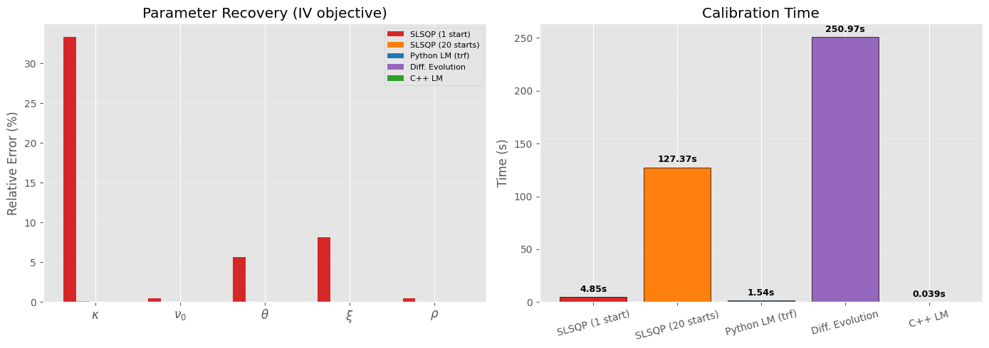
Did it find the global minimum? Yes, but with a caveat — LM is a local optimizer. It found the global minimum here because:

• This is synthetic data (true params are the global min by construction)

# IVs from all methods
def compute_ivs(params_calib):
    return [implied_vol(Heston_price_COS(S0, K_mkt[i], T_mkt[i], r, *params_calib),
                        S0, K_mkt[i], r, T_mkt[i]) for i in range(n_instruments)]

IV_lm = compute_ivs(params_lm_iv)
IV_de = compute_ivs(params_de)

IV_cpp = []
for i in range(n_instruments):
    price = cppfm.heston_call_price(S0, K_mkt[i], r, T_mkt[i],
                                     p.kappa, p.vbar, p.sigma_v, p.rho, p.v0)
    IV_cpp.append(implied_vol(price, S0, K_mkt[i], r, T_mkt[i]))

T_unique = T_maturities
K_unique = K_strikes
n_K = len(K_unique)

fig, axs = plt.subplots(1, 3, figsize=(14, 4), sharey=True)

for j, T in enumerate(T_unique):
    idx = slice(j*n_K, (j+1)*n_K)

    axs[j].scatter(K_unique, IV_mkt[idx], s=80, c='black', marker='o',
                   label='Market', zorder=3)
    axs[j].plot(K_unique, IV_iv_cos[idx], 'r-', lw=1, alpha=0.5, label='SLSQP (1 start)')
    axs[j].plot(K_unique, IV_lm[idx], 'b--', lw=1.5, label='Python LM')
    axs[j].plot(K_unique, IV_cpp[idx], 'g-', lw=2.5, marker='D',
                markersize=5, label='C++ LM')

    axs[j].set_xlabel('Strike')
    axs[j].set_title(f'T = {T}')
    axs[j].grid(True, alpha=0.3)

axs[0].set_ylabel('Implied Vol')
axs[0].legend(loc='upper right', fontsize=7)
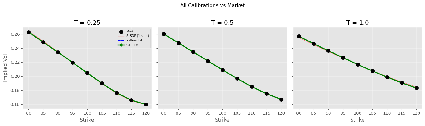
plt.suptitle('All Calibrations vs Market', y=1.02)
plt.tight_layout()
plt.show()

3.10. Hessian analysis: why kappa is hard to pin down

Assertions about “flat loss surface” need proof. The Hessian of the objective at the optimum tells us which parameter directions are well-constrained (large eigenvalues) and which are sloppy (small eigenvalues). The eigenvector associated with the smallest eigenvalue points along the valley floor.

# Hessian via finite differences at the best Python result
from scipy.optimize import approx_fprime

def hessian_fd(f, x, eps=1e-5):
    """Hessian via central finite differences."""
    n = len(x)
    H = np.zeros((n, n))
    for i in range(n):
        def gi(xi_val):
            x_copy = x.copy()
            x_copy[i] = xi_val
            return approx_fprime(x_copy, f, eps)
        g_plus = gi(x[i] + eps)
        g_minus = gi(x[i] - eps)
        H[i] = (g_plus - g_minus) / (2 * eps)
    # symmetrize
    return 0.5 * (H + H.T)

# use the best result we have (DE or LM)
params_best = params_de
H = hessian_fd(MSE_IV_COS, params_best)

eigvals, eigvecs = np.linalg.eigh(H)

print("Hessian eigenspectrum at optimum:")
print(f"{'Eigenvalue':>14}  {'Condition':>10}  Direction (kappa, nu0, theta, xi, rho)")
print("-" * 80)
for i in range(5):
    v = eigvecs[:, i]
    cond = eigvals[-1] / max(eigvals[i], 1e-20)
    # normalize for readability
    v_str = "  ".join([f"{param_names[j]}:{v[j]:+.3f}" for j in range(5)])
    print(f"{eigvals[i]:>14.2e}  {cond:>10.1f}x  [{v_str}]")

print(f"\nCondition number: {eigvals[-1] / max(eigvals[0], 1e-20):.0f}")

# which parameters dominate the flattest direction?
flat_dir = eigvecs[:, 0]
print(f"\nFlattest direction dominated by: ", end="")
sorted_idx = np.argsort(np.abs(flat_dir))[::-1]
for idx in sorted_idx[:3]:
    print(f"{param_names[idx]} ({flat_dir[idx]:+.3f})  ", end="")

# visualize: eigenvalue spectrum
fig, (ax1, ax2) = plt.subplots(1, 2, figsize=(12, 4))

ax1.bar(range(5), eigvals, color=['#d62728' if e == eigvals[0] else '#2ca02c' for e in eigvals])
ax1.set_xticks(range(5))
ax1.set_xticklabels([f'$\\lambda_{i+1}$' for i in range(5)])
ax1.set_ylabel('Eigenvalue')
ax1.set_title('Hessian Eigenspectrum')
ax1.set_yscale('log')
ax1.grid(True, alpha=0.3, axis='y')

# eigenvector heatmap
im = ax2.imshow(np.abs(eigvecs), cmap='YlOrRd', aspect='auto')
ax2.set_xticks(range(5))
ax2.set_xticklabels([f'$\\lambda_{i+1}$' for i in range(5)])
ax2.set_yticks(range(5))
ax2.set_yticklabels([r'$\kappa$', r'$\nu_0$', r'$\theta$', r'$\xi$', r'$\rho$'])
ax2.set_title('|Eigenvector| Components')
plt.colorbar(im, ax=ax2)

# annotate values
for i in range(5):
    for j in range(5):
        ax2.text(j, i, f'{eigvecs[i,j]:+.2f}', ha='center', va='center', fontsize=8,
                 color='white' if abs(eigvecs[i,j]) > 0.5 else 'black')

plt.tight_layout()
plt.show()

Hessian eigenspectrum at optimum:
    Eigenvalue   Condition  Direction (kappa, nu0, theta, xi, rho)
--------------------------------------------------------------------------------
      6.58e-06    894767.9x  [kappa:+0.998  nu0:-0.000  theta:-0.009  xi:+0.063  rho:+0.005]
      6.08e-04      9690.2x  [kappa:-0.041  nu0:-0.009  theta:+0.027  xi:+0.592  rho:+0.804]
      1.07e-02       549.3x  [kappa:+0.047  nu0:+0.002  theta:-0.050  xi:-0.801  rho:+0.594]
      3.20e-01        18.4x  [kappa:-0.012  nu0:+0.402  theta:-0.914  xi:+0.054  rho:-0.005]
      5.89e+00         1.0x  [kappa:+0.005  nu0:+0.916  theta:+0.402  xi:-0.016  rho:+0.009]

Condition number: 894768

Flattest direction dominated by: kappa (+0.998)  xi (+0.063)  theta (-0.009)  

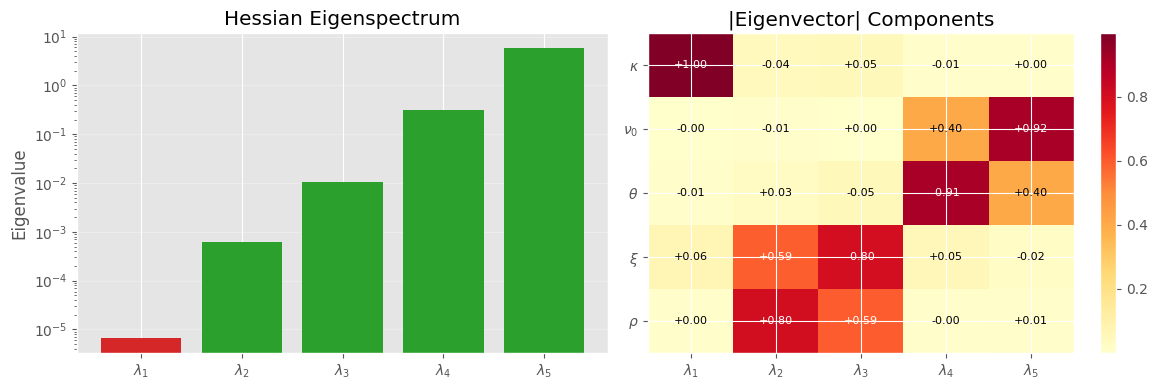
Interpretation:

• Hessian is the curvature matrix of the loss function at the optimum. Its eigenvalues tell us how steep/flat the loss surface is in each direction:

  • Large eigenvalue = steep valley -> parameter is well-identified. Moving away a tiny-bit costs a lot.

  • Small eigenvalue = nearly flat region -> parameter is poorly identified. E.g. changing kappa by a lot barely moves the loss - so the optimizer just “slides along the floor”

  • Condition number = ratio of steepest to flattest.

The heatmap:

• To see this, imagine the loss surface as a 5D bowl, not symmetric one. Each eigenvector represents a direction in the parameter space.

• Each column is an eigen-direction, each row is a parameter.

• Darker the color the parameter contributes more in that direction.

  • i.e. when the optimizer moves along that eigen-direction, that parameter is the one changing. A parameter that’s dark in a flat column (small eigenvalue) is one the data cannot control well.