11. Greeks via COS Method

COS computes Greeks through Fourier series derivatives. We validate against BS closed-form before moving to stochastic vol.

Show code cell source

Hide code cell source

import numpy as np
import matplotlib.pyplot as plt
import pandas as pd
import ipywidgets as widgets
from ipywidgets import interactive

from cos_greeks import cos_greeks_full, bs_greeks_analytical, cos_price

11.1. COS Greeks Formulas

From Fang and Oosterlee [2008], the COS option price is:

\[C = K e^{-rT} \sum_{k=0}^{N-1}\phantom{}' \text{Re}[H_k] V_k\]

where \(H_k = \varphi\left(\frac{k\pi}{b-a}\right) e^{ik\pi\frac{x_0 - a}{b-a}}\) and \(V_k\) are payoff coefficients.

Delta - differentiate w.r.t. \(S_0\) (enters through \(x_0 = \ln(S_0/K)\)):

\[\Delta = -\frac{Ke^{-rT}}{S_0} \sum_{k=0}^{N-1}\phantom{}' \omega_k \, \text{Im}[H_k] V_k\]

where \(\omega_k = \frac{k\pi}{b-a}\).

Gamma - second derivative:

\[\Gamma = \frac{Ke^{-rT}}{S_0^2} \sum_{k=0}^{N-1}\phantom{}' \left(\omega_k \, \text{Im}[H_k] - \omega_k^2 \, \text{Re}[H_k]\right) V_k\]

Theta, Vega, Rho - computed via finite differences. Analytical formulas exist but FD is simpler and accurate enough for validation.

11.2. Point Comparison: COS vs Black-Scholes

ATM call, standard parameters.

Show code cell source

Hide code cell source

# test params
S0, K, T, r, sigma = 100, 100, 1.0, 0.05, 0.2

bs = bs_greeks_analytical(S0, K, T, r, sigma, 'call')
cos = cos_greeks_full(S0, K, T, r, sigma, model='bs', N=256, L=12, opt_type='call')

# build comparison table
greeks = ['price', 'delta', 'gamma', 'theta', 'vega', 'rho']
rows = []
for g in greeks:
    bs_val = bs[g]
    cos_val = cos[g]
    err = abs(cos_val - bs_val)
    rel_err = err / abs(bs_val) if abs(bs_val) > 1e-10 else err
    rows.append([g, bs_val, cos_val, err, rel_err])

df = pd.DataFrame(rows, columns=['Greek', 'BS Analytical', 'COS Method', 'Abs Error', 'Rel Error'])
df.set_index('Greek', inplace=True)
df.style.format({'BS Analytical': '{:.6f}', 'COS Method': '{:.6f}', 'Abs Error': '{:.2e}', 'Rel Error': '{:.2e}'})

	BS Analytical	COS Method	Abs Error	Rel Error
Greek
price	10.450584	10.450584	1.78e-15	1.70e-16
delta	0.636831	0.636831	1.54e-14	2.42e-14
gamma	0.018762	0.018762	1.08e-16	5.73e-15
theta	-6.414028	-6.415077	1.05e-03	1.64e-04
vega	37.524035	37.524034	3.04e-07	8.11e-09
rho	53.232482	53.232481	7.72e-07	1.45e-08

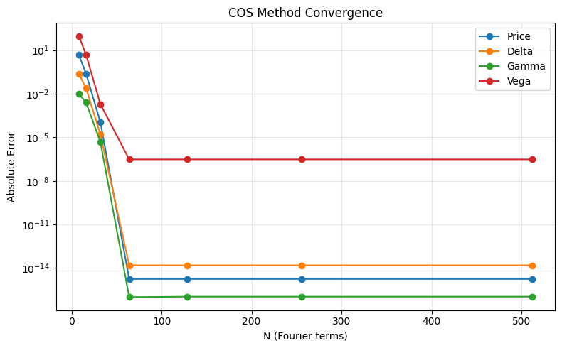
11.3. Convergence Analysis

How does error decay as we increase the number of Fourier terms N?

Show code cell source

Hide code cell source

S0, K, T, r, sigma = 100, 100, 1.0, 0.05, 0.2
bs = bs_greeks_analytical(S0, K, T, r, sigma, 'call')

N_values = [8, 16, 32, 64, 128, 256, 512]
greeks_to_plot = ['price', 'delta', 'gamma', 'vega']

errors = {g: [] for g in greeks_to_plot}
for N in N_values:
    cos = cos_greeks_full(S0, K, T, r, sigma, model='bs', N=N, L=12, opt_type='call')
    for g in greeks_to_plot:
        err = abs(cos[g] - bs[g])
        errors[g].append(err if err > 1e-16 else 1e-16)  # floor for log scale

fig, ax = plt.subplots(figsize=(8, 5))
for g in greeks_to_plot:
    ax.semilogy(N_values, errors[g], 'o-', label=g.capitalize())

ax.set_xlabel('N (Fourier terms)')
ax.set_ylabel('Absolute Error')
ax.set_title('COS Method Convergence')
ax.legend()
ax.grid(True, alpha=0.3)
plt.tight_layout()

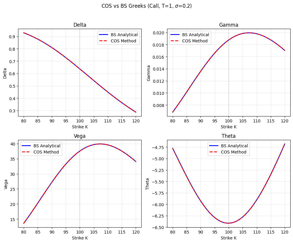
11.4. Greeks Across Strikes

Compare COS and BS Greeks for strikes from deep ITM to deep OTM.

Show code cell source

Hide code cell source

S0, T, r, sigma = 100, 1.0, 0.05, 0.2
K_range = np.linspace(80, 120, 41)

greeks_to_show = ['delta', 'gamma', 'vega', 'theta']
bs_vals = {g: [] for g in greeks_to_show}
cos_vals = {g: [] for g in greeks_to_show}

for K in K_range:
    bs = bs_greeks_analytical(S0, K, T, r, sigma, 'call')
    cos = cos_greeks_full(S0, K, T, r, sigma, model='bs', N=256, L=12, opt_type='call')
    for g in greeks_to_show:
        bs_vals[g].append(bs[g])
        cos_vals[g].append(cos[g])

fig, axes = plt.subplots(2, 2, figsize=(10, 8))
axes = axes.flatten()

for idx, g in enumerate(greeks_to_show):
    ax = axes[idx]
    ax.plot(K_range, bs_vals[g], 'b-', lw=2, label='BS Analytical')
    ax.plot(K_range, cos_vals[g], 'r--', lw=2, label='COS Method')
    ax.axvline(S0, color='gray', linestyle=':', alpha=0.5)
    ax.set_xlabel('Strike K')
    ax.set_ylabel(g.capitalize())
    ax.set_title(g.capitalize())
    ax.legend()
    ax.grid(True, alpha=0.3)

plt.suptitle('COS vs BS Greeks (Call, T=1, $\\sigma$=0.2)', y=1.02)
plt.tight_layout()

11.5. Interactive Comparison

Overlay COS and BS Greeks across spot prices. Check the match holds under different parameter regimes.

Show code cell source

Hide code cell source

def compare_greeks(K=100, T=1.0, r=0.05, sigma=0.2, opt_type='call', greek='delta'):
    S_range = np.linspace(50, 150, 51)
    
    bs_values = []
    cos_values = []
    
    for S in S_range:
        bs = bs_greeks_analytical(S, K, T, r, sigma, opt_type)
        cos = cos_greeks_full(S, K, T, r, sigma, model='bs', N=256, L=12, opt_type=opt_type)
        bs_values.append(bs[greek])
        cos_values.append(cos[greek])
    
    bs_values = np.array(bs_values)
    cos_values = np.array(cos_values)
    
    fig, (ax1, ax2) = plt.subplots(1, 2, figsize=(12, 4))
    
    # left: overlay
    ax1.plot(S_range, bs_values, 'b-', lw=2, label='BS Analytical')
    ax1.plot(S_range, cos_values, 'r--', lw=2, label='COS Method')
    ax1.axvline(K, color='gray', linestyle=':', alpha=0.7, label=f'K={K}')
    ax1.set_xlabel('Spot Price S')
    ax1.set_ylabel(greek.capitalize())
    ax1.set_title(f'{greek.capitalize()} ({opt_type})')
    ax1.legend()
    ax1.grid(True, alpha=0.3)
    
    # right: error
    error = np.abs(cos_values - bs_values)
    ax2.semilogy(S_range, error + 1e-16, 'k-', lw=1.5)
    ax2.axvline(K, color='gray', linestyle=':', alpha=0.7)
    ax2.set_xlabel('Spot Price S')
    ax2.set_ylabel('Absolute Error')
    ax2.set_title(f'{greek.capitalize()} Error')
    ax2.grid(True, alpha=0.3)
    
    plt.tight_layout()
    plt.show()
    
    # summary stats
    print(f"Max error: {error.max():.2e}, Mean error: {error.mean():.2e}")

interactive_plot = interactive(
    compare_greeks,
    K=widgets.FloatSlider(min=50, max=150, step=5, value=100, description='K'),
    T=widgets.FloatSlider(min=0.1, max=3, step=0.1, value=1.0, description='T'),
    r=widgets.FloatSlider(min=0, max=0.15, step=0.01, value=0.05, description='r'),
    sigma=widgets.FloatSlider(min=0.05, max=0.8, step=0.05, value=0.2, description='sigma'),
    opt_type=widgets.Dropdown(options=['call', 'put'], value='call', description='Type'),
    greek=widgets.Dropdown(options=['price', 'delta', 'gamma', 'theta', 'vega', 'rho'], 
                           value='delta', description='Greek')
)

display(interactive_plot)

COS matches BS Greeks to high precision (errors ~1e-6 for analytical, ~1e-4 for FD). Same code works for Heston or rough vol — just swap the characteristic function.