13. Heston Model: Hedging Under Stochastic Volatility#

Extends the BS hedging analysis to Heston. The main questions:

  • What happens when you hedge with BS deltas but reality follows Heston?

  • Does using the “correct” Heston delta actually help?

  • What risk can’t you hedge away with stock alone?

Hide code cell source

import numpy as np
import matplotlib.pyplot as plt
import sys
sys.path.insert(0, '..')

from utils import Heston_CF, Heston_price
from greeks.cos_greeks import cos_greeks_full, bs_greeks_analytical

np.random.seed(42)

13.1. Heston Model Recap#

Under Heston [Heston, 1993], stock and variance follow:

\[dS_t = r S_t \, dt + \sqrt{v_t} S_t \, dW_t^S\]
\[dv_t = \kappa(\theta - v_t) \, dt + \xi \sqrt{v_t} \, dW_t^v\]

with \(\text{Corr}(dW^S, dW^v) = \rho\).

The parameters: \(v_0\) is initial variance, \(\theta\) is long-run variance, \(\kappa\) controls mean-reversion speed, \(\xi\) is vol-of-vol, and \(\rho\) is typically negative (the leverage effect—when stock drops, vol tends to rise).

For hedging, the key difference from BS is that volatility is now a second source of randomness. Option prices depend on the current vol level, and that level moves around.

Hide code cell source

# Heston parameters
S0 = 100
K = 100
T = 0.25
r = 0.05

v0 = 0.04        # Initial variance (vol = 20%)
theta = 0.04     # Long-run variance
kappa = 2.0      # Mean-reversion speed
xi = 0.3         # Vol-of-vol
rho = -0.7       # Correlation (leverage effect)

sigma_bs = np.sqrt(v0)  # Equivalent BS vol for comparison

print("Model Parameters")
print("="*40)
print(f"Spot S0:          {S0}")
print(f"Strike K:         {K}")
print(f"Time T:           {T} years")
print(f"Risk-free r:      {r}")
print(f"Initial vol:      {100*np.sqrt(v0):.1f}%")
print(f"Long-run vol:     {100*np.sqrt(theta):.1f}%")
print(f"Vol-of-vol xi:    {xi}")
print(f"Correlation rho:  {rho}")
Model Parameters
========================================
Spot S0:          100
Strike K:         100
Time T:           0.25 years
Risk-free r:      0.05
Initial vol:      20.0%
Long-run vol:     20.0%
Vol-of-vol xi:    0.3
Correlation rho:  -0.7

13.2. Heston Greeks via COS Method#

Under Heston, Greeks need to be computed numerically. We use the COS method [Fang and Oosterlee, 2008]—analytical derivatives for delta/gamma, finite differences for vega and theta.

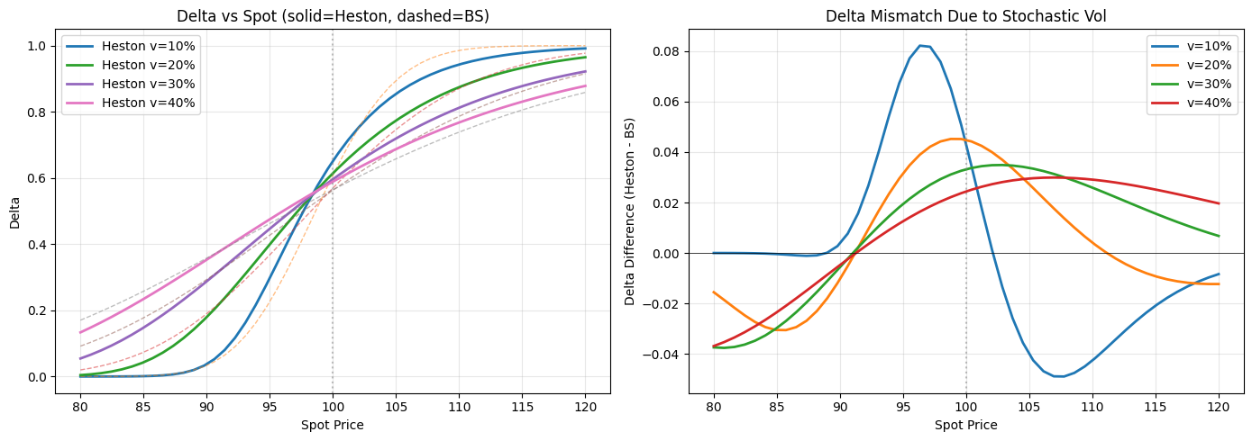
The important difference from BS: Heston delta depends on the current variance \(v_t\), not just spot. Even if spot doesn’t move, delta changes as vol moves around.

Hide code cell source

# Compare BS vs Heston Greeks
bs_g = bs_greeks_analytical(S0, K, T, r, sigma_bs, 'call')
heston_g = cos_greeks_full(S0, K, T, r, v0, model='heston', N=256, L=12,
                           opt_type='call', heston_cf=Heston_CF,
                           kappa=kappa, theta=theta, xi=xi, rho=rho)

print("Greeks Comparison: BS vs Heston")
print("="*50)
print(f"{'Greek':<12} {'BS':>12} {'Heston':>12} {'Diff %':>12}")
print("-"*50)
for g in ['price', 'delta', 'gamma', 'theta', 'vega']:
    bs_val = bs_g[g]
    h_val = heston_g[g]
    diff_pct = 100 * (h_val - bs_val) / abs(bs_val) if bs_val != 0 else 0
    print(f"{g.capitalize():<12} {bs_val:>12.6f} {h_val:>12.6f} {diff_pct:>11.2f}%")
Greeks Comparison: BS vs Heston
==================================================
Greek                  BS       Heston       Diff %
--------------------------------------------------
Price            4.614997     4.587070       -0.61%
Delta            0.569460     0.614251        7.87%
Gamma            0.039288     0.038115       -2.99%
Theta          -10.474151   -10.361430        1.08%
Vega            19.644000    15.375729      -21.73%

Hide code cell source

# Delta as function of spot and vol
spots = np.linspace(80, 120, 50)
vols = [0.01, 0.04, 0.09, 0.16]  # 10%, 20%, 30%, 40%

fig, axes = plt.subplots(1, 2, figsize=(14, 5))

# Left: Delta vs Spot for different vol levels
ax = axes[0]
for v in vols:
    deltas_heston = []
    deltas_bs = []
    for s in spots:
        h_g = cos_greeks_full(s, K, T, r, v, model='heston', N=256, L=12,
                              heston_cf=Heston_CF, kappa=kappa, theta=theta, xi=xi, rho=rho)
        b_g = bs_greeks_analytical(s, K, T, r, np.sqrt(v), 'call')
        deltas_heston.append(h_g['delta'])
        deltas_bs.append(b_g['delta'])
    ax.plot(spots, deltas_heston, '-', label=f'Heston v={100*np.sqrt(v):.0f}%', linewidth=2)
    ax.plot(spots, deltas_bs, '--', alpha=0.5, linewidth=1)

ax.axvline(K, color='gray', linestyle=':', alpha=0.5)
ax.set_xlabel('Spot Price')
ax.set_ylabel('Delta')
ax.set_title('Delta vs Spot (solid=Heston, dashed=BS)')
ax.legend()
ax.grid(True, alpha=0.3)

# Right: Delta difference (Heston - BS)
ax = axes[1]
for v in vols:
    delta_diff = []
    for s in spots:
        h_g = cos_greeks_full(s, K, T, r, v, model='heston', N=256, L=12,
                              heston_cf=Heston_CF, kappa=kappa, theta=theta, xi=xi, rho=rho)
        b_g = bs_greeks_analytical(s, K, T, r, np.sqrt(v), 'call')
        delta_diff.append(h_g['delta'] - b_g['delta'])
    ax.plot(spots, delta_diff, '-', label=f'v={100*np.sqrt(v):.0f}%', linewidth=2)

ax.axhline(0, color='k', linestyle='-', linewidth=0.5)
ax.axvline(K, color='gray', linestyle=':', alpha=0.5)
ax.set_xlabel('Spot Price')
ax.set_ylabel('Delta Difference (Heston - BS)')
ax.set_title('Delta Mismatch Due to Stochastic Vol')
ax.legend()
ax.grid(True, alpha=0.3)

plt.tight_layout()
plt.show()
../_images/c91dec74dd1756f6bb5e4fd3932dc5b574d8e78f1724ff1b32fcf1ed6817d501.png

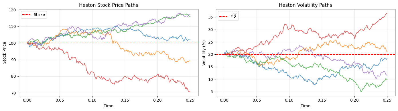
13.3. Simulating Heston Paths#

We use Euler discretization:

\[S_{t+\Delta t} = S_t \exp\left[(r - \tfrac{1}{2}v_t)\Delta t + \sqrt{v_t}\sqrt{\Delta t}\, Z_1\right]\]
\[v_{t+\Delta t} = v_t + \kappa(\theta - v_t)\Delta t + \xi\sqrt{v_t}\sqrt{\Delta t}\, Z_2\]

where \(Z_1\) and \(Z_2\) are correlated normals with \(\text{Corr}(Z_1, Z_2) = \rho\).

Hide code cell source

def simulate_heston_path(S0, v0, r, kappa, theta, xi, rho, T, n_steps):
    """Euler discretization of Heston model."""
    dt = T / n_steps
    sqrt_dt = np.sqrt(dt)
    
    S = np.zeros(n_steps + 1)
    v = np.zeros(n_steps + 1)
    S[0], v[0] = S0, v0
    
    for i in range(n_steps):
        # Correlated Brownians
        z1 = np.random.randn()
        z2 = rho * z1 + np.sqrt(1 - rho**2) * np.random.randn()
        
        # Variance (with reflection to keep positive)
        v_curr = max(v[i], 0)
        sqrt_v = np.sqrt(v_curr)
        v[i+1] = v_curr + kappa * (theta - v_curr) * dt + xi * sqrt_v * sqrt_dt * z2
        v[i+1] = max(v[i+1], 1e-8)
        
        # Stock price
        S[i+1] = S[i] * np.exp((r - 0.5 * v_curr) * dt + sqrt_v * sqrt_dt * z1)
    
    times = np.linspace(0, T, n_steps + 1)
    return times, S, v

Hide code cell source

# Show example Heston paths
fig, axes = plt.subplots(1, 2, figsize=(14, 4))

np.random.seed(123)
for _ in range(5):
    times, S, v = simulate_heston_path(S0, v0, r, kappa, theta, xi, rho, T, 252)
    axes[0].plot(times, S, alpha=0.7)
    axes[1].plot(times, 100*np.sqrt(v), alpha=0.7)

axes[0].axhline(K, color='r', linestyle='--', label='Strike')
axes[0].set_xlabel('Time')
axes[0].set_ylabel('Stock Price')
axes[0].set_title('Heston Stock Price Paths')
axes[0].legend()
axes[0].grid(True, alpha=0.3)

axes[1].axhline(100*np.sqrt(theta), color='r', linestyle='--', label=r'$\sqrt{\theta}$')
axes[1].set_xlabel('Time')
axes[1].set_ylabel('Volatility (%)')
axes[1].set_title('Heston Volatility Paths')
axes[1].legend()
axes[1].grid(True, alpha=0.3)

plt.tight_layout()
plt.show()
../_images/0c3a8c9af14f461db81d5ba09d6b6d150c24688fe81728b5e71ad9b64b512e39.png

13.4. BS Delta vs Heston Delta#

Here’s the experiment: reality follows Heston, we sell an option and delta-hedge. We compare hedging with BS delta (using \(\sigma = \sqrt{v_t}\)) vs the full Heston delta.

Both methods observe the true variance at each hedge time. The question is whether knowing the full Heston dynamics—mean-reversion, vol-of-vol, correlation—actually improves the hedge.

We expect the unhedgeable vol risk to dominate the delta choice — let’s see.

Hide code cell source

def hedge_under_heston(S0, K, T, r, v0, kappa, theta, xi, rho, n_hedge, hedge_model='heston'):
    """ Delta-hedge a short call under Heston dynamics.
    hedge_model: 'heston' uses Heston delta, 'bs' uses BS delta with sqrt(v_t)
    """
    dt = T / n_hedge
    
    # Simulate Heston path
    times, S, v = simulate_heston_path(S0, v0, r, kappa, theta, xi, rho, T, n_hedge)
    
    # Initial option price (Heston price - this is what we receive)
    V0 = Heston_price(S0, K, T, r, kappa, v0, theta, xi, rho)
    
    # Get initial delta
    if hedge_model == 'heston':
        g = cos_greeks_full(S0, K, T, r, v0, model='heston', N=256, L=12,
                            heston_cf=Heston_CF, kappa=kappa, theta=theta, xi=xi, rho=rho)
        delta = g['delta']
    else:  # BS
        g = bs_greeks_analytical(S0, K, T, r, np.sqrt(v0), 'call')
        delta = g['delta']
    
    shares = delta
    cash = V0 - delta * S0
    
    portfolio_values = [V0]
    deltas_used = [delta]
    
    for i in range(1, n_hedge + 1):

        tau = T - times[i]
        cash *= np.exp(r * dt)
        
        portfolio_value = shares * S[i] + cash
        
        # Get new delta
        if tau > 1e-6:
            if hedge_model == 'heston':
                g = cos_greeks_full(S[i], K, tau, r, v[i], model='heston', N=256, L=12,
                                    heston_cf=Heston_CF, kappa=kappa, theta=theta, xi=xi, rho=rho)
                new_delta = g['delta']
            else:  # BS with current vol
                g = bs_greeks_analytical(S[i], K, tau, r, np.sqrt(v[i]), 'call')
                new_delta = g['delta']
        else:
            new_delta = 1.0 if S[i] > K else 0.0
        
        # Rebalance
        shares_traded = new_delta - shares
        cash -= shares_traded * S[i]
        shares = new_delta
        
        portfolio_values.append(portfolio_value)
        deltas_used.append(new_delta)
    
    # Final PnL
    payoff = max(S[-1] - K, 0)
    final_portfolio = shares * S[-1] + cash
    hedge_pnl = final_portfolio - payoff
    
    return {
        'times': times,
        'spot': S,
        'vol': v,
        'portfolio_values': np.array(portfolio_values),
        'deltas': np.array(deltas_used),
        'hedge_pnl': hedge_pnl,
        'payoff': payoff,
        'final_portfolio': final_portfolio
    }

Hide code cell source

# Run Monte Carlo comparison
n_paths = 500
n_hedge = 50

pnl_bs = []
pnl_heston = []

print("Running hedge comparison...")
for i in range(n_paths):
    np.random.seed(i)  # Same paths for fair comparison
    res_bs = hedge_under_heston(S0, K, T, r, v0, kappa, theta, xi, rho, n_hedge, 'bs')
    
    np.random.seed(i)
    res_h = hedge_under_heston(S0, K, T, r, v0, kappa, theta, xi, rho, n_hedge, 'heston')
    
    pnl_bs.append(res_bs['hedge_pnl'])
    pnl_heston.append(res_h['hedge_pnl'])

pnl_bs = np.array(pnl_bs)
pnl_heston = np.array(pnl_heston)

print("\nHedge PnL Statistics")
print("="*60)
print(f"{'Metric':<20} {'BS Delta':>18} {'Heston Delta':>18}")
print("-"*60)
print(f"{'Mean PnL':<20} {np.mean(pnl_bs):>18.4f} {np.mean(pnl_heston):>18.4f}")
print(f"{'Std PnL':<20} {np.std(pnl_bs):>18.4f} {np.std(pnl_heston):>18.4f}")
print(f"{'5th Percentile':<20} {np.percentile(pnl_bs, 5):>18.4f} {np.percentile(pnl_heston, 5):>18.4f}")
print(f"{'95th Percentile':<20} {np.percentile(pnl_bs, 95):>18.4f} {np.percentile(pnl_heston, 95):>18.4f}")
Running hedge comparison...
Hedge PnL Statistics
============================================================
Metric                         BS Delta       Heston Delta
------------------------------------------------------------
Mean PnL                        -0.0424            -0.0433
Std PnL                          0.8005             0.8826
5th Percentile                  -1.5596            -1.6255
95th Percentile                  1.1424             1.1698
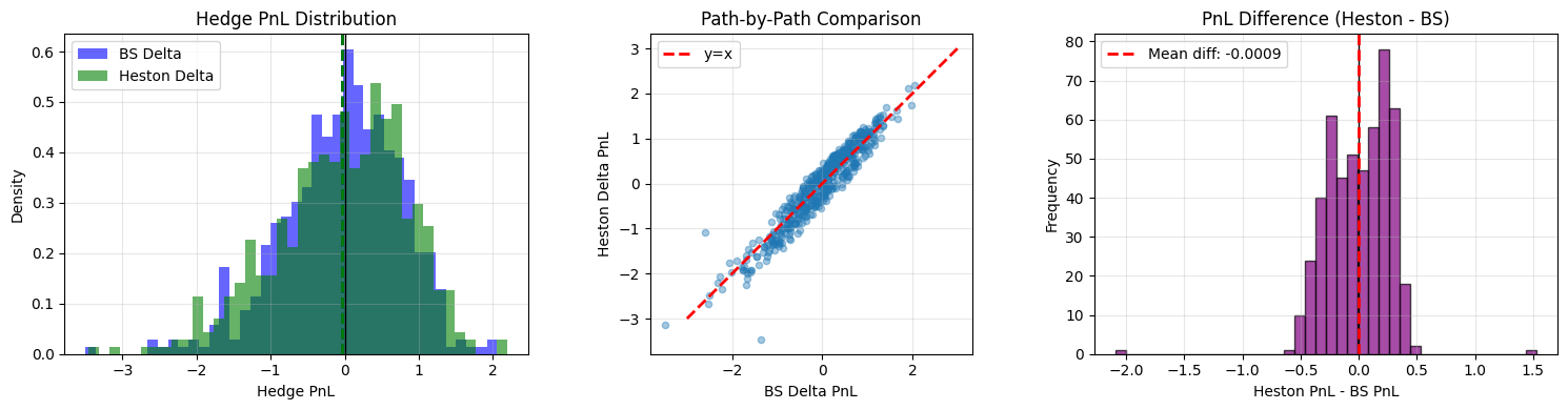
Hide code cell source

fig, axes = plt.subplots(1, 3, figsize=(15, 4))

# PnL distributions
ax = axes[0]
ax.hist(pnl_bs, bins=40, alpha=0.6, label='BS Delta', density=True, color='blue')
ax.hist(pnl_heston, bins=40, alpha=0.6, label='Heston Delta', density=True, color='green')
ax.axvline(np.mean(pnl_bs), color='blue', linestyle='--', linewidth=2)
ax.axvline(np.mean(pnl_heston), color='green', linestyle='--', linewidth=2)
ax.axvline(0, color='k', linestyle='-', linewidth=1)
ax.set_xlabel('Hedge PnL')
ax.set_ylabel('Density')
ax.set_title('Hedge PnL Distribution')
ax.legend()
ax.grid(True, alpha=0.3)

# Scatter: BS vs Heston PnL
ax = axes[1]
ax.scatter(pnl_bs, pnl_heston, alpha=0.4, s=20)
ax.plot([-3, 3], [-3, 3], 'r--', linewidth=2, label='y=x')
ax.set_xlabel('BS Delta PnL')
ax.set_ylabel('Heston Delta PnL')
ax.set_title('Path-by-Path Comparison')
ax.legend()
ax.grid(True, alpha=0.3)
ax.set_aspect('equal')

# PnL difference distribution
ax = axes[2]
pnl_diff = pnl_heston - pnl_bs
ax.hist(pnl_diff, bins=40, alpha=0.7, color='purple', edgecolor='black')
ax.axvline(0, color='k', linestyle='-', linewidth=1)
ax.axvline(np.mean(pnl_diff), color='r', linestyle='--', linewidth=2, 
           label=f'Mean diff: {np.mean(pnl_diff):.4f}')
ax.set_xlabel('Heston PnL - BS PnL')
ax.set_ylabel('Frequency')
ax.set_title('PnL Difference (Heston - BS)')
ax.legend()
ax.grid(True, alpha=0.3)

plt.tight_layout()
plt.show()

print(f"\nKey Finding:")
print(f"  BS Delta std:     {np.std(pnl_bs):.4f}")
print(f"  Heston Delta std: {np.std(pnl_heston):.4f}")
print(f"  Correlation:      {np.corrcoef(pnl_bs, pnl_heston)[0,1]:.4f}")
print(f"\nThe high correlation shows both methods face the SAME underlying risk: vol moves.")
../_images/a6ad7567de13b37bef47931c55bb1beb5e79f3db20f0a637cca6ebce0bccf107.png
Key Finding:
  BS Delta std:     0.8005
  Heston Delta std: 0.8826
  Correlation:      0.9530

The high correlation shows both methods face the SAME underlying risk: vol moves.

PnL from both methods is highly correlated — the unhedgeable vol risk dominates the delta choice. Model choice matters more for exotics with strong path-dependence.

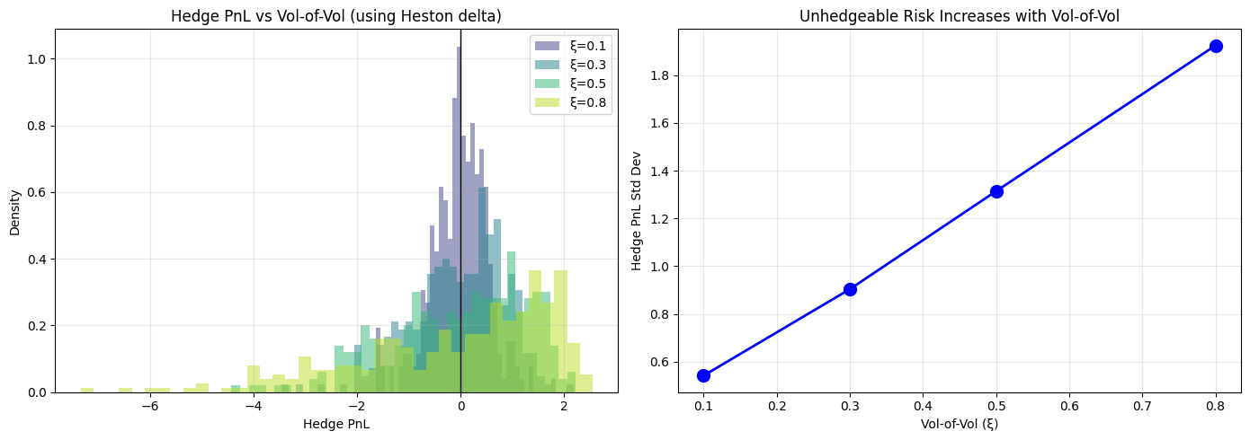
13.5. The Unhedgeable Risk: Vol-of-Vol#

Even with the correct Heston delta, risk remains. The option value depends on two state variables, \(V = V(S_t, v_t, t)\), and the delta-hedged PnL is:

\[d\Pi = \frac{\partial V}{\partial v} dv + \frac{1}{2}\frac{\partial^2 V}{\partial S^2}(dS)^2 + \frac{\partial V}{\partial t}dt\]

Stock hedges the \(dS\) risk. But the \(dv\) term—exposure to variance moves—requires other instruments: variance swaps, VIX options, or other vanilla options.

With only stock, the \(dv\) exposure remains. And this exposure scales with \(\xi\) (vol-of-vol): higher \(\xi\) means more variance in variance, means more unhedgeable risk.

Hide code cell source

# Test different vol-of-vol levels
xi_values = [0.1, 0.3, 0.5, 0.8]
n_paths_xi = 300

results_xi = {}

print("Testing vol-of-vol impact...")
for xi_test in xi_values:
    pnls = []
    for i in range(n_paths_xi):
        np.random.seed(i)
        res = hedge_under_heston(S0, K, T, r, v0, kappa, theta, xi_test, rho, n_hedge, 'heston')
        pnls.append(res['hedge_pnl'])
    results_xi[xi_test] = np.array(pnls)
    print(f"  xi={xi_test:.1f}: std={np.std(pnls):.4f}")
Testing vol-of-vol impact...
  xi=0.1: std=0.5416
  xi=0.3: std=0.9037
  xi=0.5: std=1.3142
  xi=0.8: std=1.9244

Hide code cell source

fig, axes = plt.subplots(1, 2, figsize=(14, 5))

# PnL distributions for different xi
ax = axes[0]
colors = plt.cm.viridis(np.linspace(0.2, 0.9, len(xi_values)))
for xi_test, color in zip(xi_values, colors):
    ax.hist(results_xi[xi_test], bins=40, alpha=0.5, label=f'ξ={xi_test}', 
            density=True, color=color)
ax.axvline(0, color='k', linestyle='-', linewidth=1)
ax.set_xlabel('Hedge PnL')
ax.set_ylabel('Density')
ax.set_title('Hedge PnL vs Vol-of-Vol (using Heston delta)')
ax.legend()
ax.grid(True, alpha=0.3)

# Std vs xi
ax = axes[1]
stds = [np.std(results_xi[xi]) for xi in xi_values]
ax.plot(xi_values, stds, 'bo-', linewidth=2, markersize=10)
ax.set_xlabel('Vol-of-Vol (ξ)')
ax.set_ylabel('Hedge PnL Std Dev')
ax.set_title('Unhedgeable Risk Increases with Vol-of-Vol')
ax.grid(True, alpha=0.3)

plt.tight_layout()
plt.show()
../_images/d08c54da58b33068e45c90784e4d98bb732d0b2b28f6c81e2349f29d2cfd8e78.png

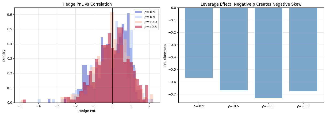
13.6. The Leverage Effect#

The correlation \(\rho\) between stock returns and variance creates the leverage effect: when stock drops, vol tends to rise (\(\rho < 0\)). This creates negatively-skewed returns—the left tail is fatter.

For hedging, this is bad news. Large down moves coincide with vol spikes, so your hedge deteriorates exactly when you need it most. The PnL distribution becomes negatively skewed.

Hide code cell source

# Compare different correlations
rho_values = [-0.9, -0.5, 0.0, 0.5]
n_paths_rho = 300

results_rho = {}

print("Testing correlation impact...")
for rho_test in rho_values:
    pnls = []
    for i in range(n_paths_rho):
        np.random.seed(i)
        res = hedge_under_heston(S0, K, T, r, v0, kappa, theta, xi, rho_test, n_hedge, 'heston')
        pnls.append(res['hedge_pnl'])
    results_rho[rho_test] = np.array(pnls)
    print(f"  rho={rho_test:+.1f}: mean={np.mean(pnls):.4f}, std={np.std(pnls):.4f}")
Testing correlation impact...
  rho=-0.9: mean=-0.0420, std=0.8852
  rho=-0.5: mean=-0.0362, std=0.9147
  rho=+0.0: mean=-0.0349, std=0.9318
  rho=+0.5: mean=-0.0146, std=0.9282

Hide code cell source

fig, axes = plt.subplots(1, 2, figsize=(14, 5))

ax = axes[0]
colors = plt.cm.coolwarm(np.linspace(0, 1, len(rho_values)))
for rho_test, color in zip(rho_values, colors):
    ax.hist(results_rho[rho_test], bins=40, alpha=0.5, label=f'ρ={rho_test:+.1f}', 
            density=True, color=color)
ax.axvline(0, color='k', linestyle='-', linewidth=1)
ax.set_xlabel('Hedge PnL')
ax.set_ylabel('Density')
ax.set_title('Hedge PnL vs Correlation')
ax.legend()
ax.grid(True, alpha=0.3)

# Skewness vs rho
from scipy.stats import skew
ax = axes[1]
skews = [skew(results_rho[r]) for r in rho_values]
stds = [np.std(results_rho[r]) for r in rho_values]

ax.bar(range(len(rho_values)), skews, color='steelblue', alpha=0.7)
ax.set_xticks(range(len(rho_values)))
ax.set_xticklabels([f'ρ={r:+.1f}' for r in rho_values])
ax.axhline(0, color='k', linestyle='-', linewidth=0.5)
ax.set_ylabel('PnL Skewness')
ax.set_title('Leverage Effect: Negative ρ Creates Negative Skew')
ax.grid(True, alpha=0.3, axis='y')

plt.tight_layout()
plt.show()
../_images/d7f8029dec053b8adf9cb9c05db87ffbe9ebda55c08343296303938fd81934a5.png

For vanilla hedging, BS delta with current vol works nearly as well as Heston delta. The dominant risk is vol moves, which stock can’t hedge — need variance swaps or other options for that.

TODO: add vega hedging with a second option to quantify how much residual risk drops.