2. Exact Heston Model Simulations for Characteristic Function Methods

2.1. Overview

Exact simulation from Broadie and Kaya [2006]. All implementations in utils.py.

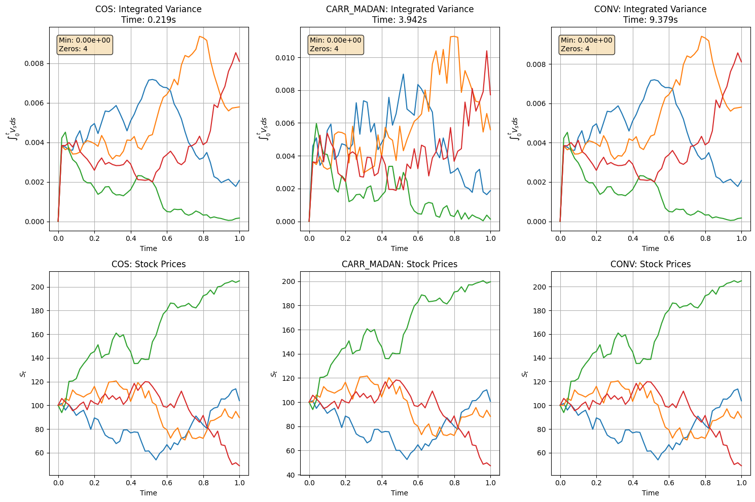
The critical step is inverting the CDF of integrated variance \(\int_0^T V_s \, ds\). We compare COS, Carr-Madan, and CONV for that inversion.

Show code cell source

Hide code cell source

import sys
sys.path.insert(0, '..')
from utils import *

Show code cell source

Hide code cell source

# Parameters
NoOfPaths = 4
NoOfSteps = 50

# Heston model parameters
gamma = 0.4 # vol of vol
kappa = 0.5 # speed of mean reversion
vbar = 0.2 # long-term mean
rho = -0.9 # negative correlation
v0 = 0.2 # initial variance
T = 1.0
S_0 = 100.0
r = 0.1

nr_expansion = 100
L = 10

# Set random seed for reproducibility
np.random.seed(3)

# Test all three methods
methods_to_test = {
    "cos": {},
    "carr_madan": {"N": 2**12},
    "conv": {"alpha": 0.5, "N": 2**13}
}

results = {}

for method_name, kwargs in methods_to_test.items():
    print(f"\n=== Testing {method_name.upper()} Method ===")
    
    # Reset random seed to ensure fair comparison
    np.random.seed(3)
    
    start_time = time.time()
    paths = GeneratePathsHestonES(
        NoOfPaths, NoOfSteps, T, r, S_0, kappa, gamma, rho, vbar, v0,
        nr_expansion=nr_expansion, L=L, recovery_method=method_name, **kwargs
    )
    end_time = time.time()
    
    results[method_name] = {
        "paths": paths,
        "computation_time": end_time - start_time
    }
    
    # Check for zeros in integrated variance
    V_int = paths["Vint"]
    min_vint = np.min(V_int)
    zero_count = np.sum(V_int <= 1e-10)
    
    print(f"Computation time: {end_time - start_time:.3f} seconds")
    print(f"Min integrated variance: {min_vint:.8f}")
    print(f"Values <= 1e-10: {zero_count}/{V_int.size}")
    print(f"All positive: {np.all(V_int > 0)}")

# Plot comparison
fig, axes = plt.subplots(2, 3, figsize=(15, 10))

for idx, (method_name, result) in enumerate(results.items()):
    timeGrid = result["paths"]["time"]
    S = result["paths"]["S"]
    V_int = result["paths"]["Vint"]
    
    # Plot integrated variance
    axes[0, idx].grid(True)
    axes[0, idx].plot(timeGrid, np.transpose(V_int))
    axes[0, idx].set_xlabel('Time')
    axes[0, idx].set_ylabel(r'$\int_0^t V_s ds$')
    axes[0, idx].set_title(f'{method_name.upper()}: Integrated Variance\nTime: {result["computation_time"]:.3f}s')
    
    # Add text showing min value and zero count
    min_val = np.min(V_int)
    zero_count = np.sum(V_int <= 1e-10)
    axes[0, idx].text(0.05, 0.95, f'Min: {min_val:.2e}\nZeros: {zero_count}', 
                     transform=axes[0, idx].transAxes, verticalalignment='top',
                     bbox=dict(boxstyle='round', facecolor='wheat', alpha=0.8))
    
    # Plot stock price paths
    axes[1, idx].grid(True)
    axes[1, idx].plot(timeGrid, np.transpose(S))
    axes[1, idx].set_xlabel('Time')
    axes[1, idx].set_ylabel(r'$S_t$')
    axes[1, idx].set_title(f'{method_name.upper()}: Stock Prices')

plt.tight_layout()
plt.show()

# Print timing comparison
print("\n=== Performance Comparison ===")
for method_name, result in results.items():
    print(f"{method_name.upper()}: {result['computation_time']:.3f} seconds")

# Print zero analysis
print("\n=== Zero Analysis ===") # 4 zeros since we start from 0 for each path, 4 paths give 4 0s
for method_name, result in results.items():
    V_int = result["paths"]["Vint"]
    min_val = np.min(V_int)
    zero_count = np.sum(V_int <= 1e-10)
    exact_zero_count = np.sum(V_int == 0.0)
    print(f"{method_name.upper()}: min={min_val:.8f}, zeros(<=1e-10)={zero_count}, exact_zeros={exact_zero_count}")

=== Testing COS Method ===
Using cos method for CDF recovery and inversion

Computation time: 0.219 seconds
Min integrated variance: 0.00000000
Values <= 1e-10: 4/204
All positive: False

=== Testing CARR_MADAN Method ===
Using carr_madan method for CDF recovery and inversion

Computation time: 3.942 seconds
Min integrated variance: 0.00000000
Values <= 1e-10: 4/204
All positive: False

=== Testing CONV Method ===
Using conv method for CDF recovery and inversion

Computation time: 9.379 seconds
Min integrated variance: 0.00000000
Values <= 1e-10: 4/204
All positive: False

=== Performance Comparison ===
COS: 0.219 seconds
CARR_MADAN: 3.942 seconds
CONV: 9.379 seconds

=== Zero Analysis ===
COS: min=0.00000000, zeros(<=1e-10)=4, exact_zeros=4
CARR_MADAN: min=0.00000000, zeros(<=1e-10)=4, exact_zeros=4
CONV: min=0.00000000, zeros(<=1e-10)=4, exact_zeros=4

Show code cell source

Hide code cell source

np.random.seed(19937)
paths = GeneratePathsHestonES(
    NoOfPaths=3, NoOfSteps=10, T=0.5, r=0.05, S_0=100,
    kappa=0.5, gamma=0.4, rho=-0.7, vbar=0.2, v0=0.2,
    nr_expansion=50, L=8, recovery_method='carr_madan', N=2048
)

min_vint = np.min(paths['Vint'])
zero_count = np.sum(paths['Vint'] < 1e-10)
print(f"Min integrated variance: {min_vint:.8f}")
print(f"Zero values: {zero_count}/{paths['Vint'].size}")
print(f"All values positive: {np.all(paths['Vint'] > 0)}")

# Show first few values
print(f"First few values: {paths['Vint'][:, :5]}")

# If we still see zeros, there's a problem with the import
if zero_count > 0:
    print("ERROR: Still seeing zeros! The fixed utils.py is not being used.")
    print("Please restart the Jupyter kernel and run all cells again.")
else:
    print("SUCCESS: No zeros found! The fix is working correctly.")

Using carr_madan method for CDF recovery and inversion

Min integrated variance: 0.00000000
Zero values: 3/33
All values positive: False
First few values: [[0.         0.00820748 0.01244008 0.0057766  0.00594041]
 [0.         0.01216603 0.00488742 0.00421274 0.00721754]
 [0.         0.01324573 0.00684682 0.00610527 0.01005191]]
ERROR: Still seeing zeros! The fixed utils.py is not being used.
Please restart the Jupyter kernel and run all cells again.

COS is fastest since it avoids numerical integration. Carr-Madan occasionally produces near-zero PDFs that break Newton’s method — need to investigate. All three produce similar stock trajectories, the difference is in the variance sampling step.

2.2. Comparison

COS for this application — fast, stable, no integration needed.

2.2.1. Newton-Raphson method vs. brute force approach for CDF inversion

Show code cell source

Hide code cell source

compare_cdf_inversion_methods()

/home/runner/work/Quantitative-Finance-Book/Quantitative-Finance-Book/char_functions/../utils.py:502: RuntimeWarning: invalid value encountered in scalar multiply
  chf = temp1 * temp2 * temp3 / temp4
/home/runner/work/Quantitative-Finance-Book/Quantitative-Finance-Book/char_functions/../utils.py:502: RuntimeWarning: invalid value encountered in scalar divide
  chf = temp1 * temp2 * temp3 / temp4
/home/runner/work/Quantitative-Finance-Book/Quantitative-Finance-Book/char_functions/../utils.py:468: RuntimeWarning: invalid value encountered in divide
  R
/home/runner/work/Quantitative-Finance-Book/Quantitative-Finance-Book/char_functions/../utils.py:479: RuntimeWarning: invalid value encountered in divide
  - R * (1 + np.exp(-R * tau)) / (1 - np.exp(-R * tau))
/home/runner/work/Quantitative-Finance-Book/Quantitative-Finance-Book/char_functions/../utils.py:486: RuntimeWarning: invalid value encountered in divide
  np.sqrt(vt * vu)

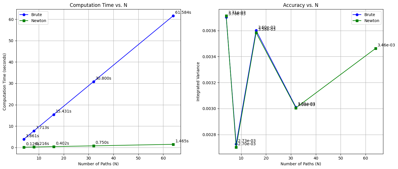
	N	Brute Time (s)	Newton Time (s)	vint_brute_values	vint_newton_values
0	4	3.860675	0.125718	0.003704	0.003713
1	8	7.712639	0.215924	0.002726	0.002702
2	16	15.431197	0.402222	0.003600	0.003583
3	32	30.799817	0.750099	0.003011	0.003005
4	64	61.583629	1.465462	NaN	0.003462