8. Pricing American Options by Finite Difference

• Replicating the Finite Difference implementation in [Longstaff and Schwartz, 2001].

• Replicating the values in Table 1.

• Completely replicating the Table 1, as in the paper (last cell of the code)

8.1. Background

The Black-Scholes PDE for a derivative \(V(S,t)\) is:

\[\frac{\partial V}{\partial t} + \frac{1}{2}\sigma^2 S^2 \frac{\partial^2 V}{\partial S^2} + rS\frac{\partial V}{\partial S} - rV = 0\]

Log-transformation: Setting \(X = \log(S)\) simplifies to constant coefficients:

\[\frac{\partial V}{\partial t} + \frac{1}{2}\sigma^2 \frac{\partial^2 V}{\partial X^2} + \left(r - \frac{1}{2}\sigma^2\right)\frac{\partial V}{\partial X} - rV = 0\]

Discretization schemes:

• European (FTCS): Forward in time, central in space - explicit scheme

• American (BTCS): Backward in time, central in space - implicit scheme with early exercise constraint

For American options, at each time step we enforce: \(V \geq \max(K - S, 0)\)

Show code cell source

Hide code cell source

import numpy as np
from scipy.stats import norm
from scipy.sparse import diags, eye as speye
from scipy.sparse.linalg import splu
import pandas as pd
import matplotlib.pyplot as plt
import time
import sys
sys.path.insert(0, '..')
from utils import bs_put_price

8.2. LSMC Helper Functions

We define the LSMC pricer from Longstaff and Schwartz [2001] here for benchmarking the finite difference results.

Show code cell source

Hide code cell source

# GBM with antithetic sampling
# generate Z step-by-step -> halves peak memory
def simulate_gbm_paths(S0, r, sigma, T, n_steps, n_paths):
    np.random.seed(1)
    dt = T / n_steps
    drift = (r - 0.5 * sigma**2) * dt
    diffusion = sigma * np.sqrt(dt)
    
    n_total = 2 * n_paths
    S = np.zeros((n_total, n_steps + 1))
    S[:, 0] = S0
    
    for t in range(n_steps):
        Z = np.random.randn(n_paths)
        S[:n_paths, t+1] = S[:n_paths, t] * np.exp(drift + diffusion * Z)
        S[n_paths:, t+1] = S[n_paths:, t] * np.exp(drift - diffusion * Z)
    return S


# weighted Laguerre polynomials, scaled by moneyness
def laguerre_polynomials(x, K):
    x_scaled = x / K
    exp_term = np.exp(-x_scaled / 2)
    L0 = exp_term
    L1 = exp_term * (1 - x_scaled)
    L2 = exp_term * (1 - 2*x_scaled + x_scaled**2 / 2)
    return L0, L1, L2


# LSMC pricer - backward induction with regression for continuation value
def lsmc_american_put(S, K, r, T, n_steps):
    n_paths = S.shape[0]
    dt = T / n_steps
    df = np.exp(-r * dt)
    
    cash_flows = np.zeros((n_paths, n_steps + 1))
    cash_flows[:, -1] = np.maximum(K - S[:, -1], 0)
    
    for t in range(n_steps - 1, 0, -1):
        payoff = np.maximum(K - S[:, t], 0)
        itm = payoff > 0
        
        if np.sum(itm) > 0:
            X = S[itm, t]
            L0, L1, L2 = laguerre_polynomials(X, K)
            A = np.column_stack([np.ones_like(X), L0, L1, L2])
            
            # discounted future CFs -> Y for regression
            Y = np.zeros(n_paths)
            for s in range(t+1, n_steps+1):
                Y += cash_flows[:, s] * df**(s-t)
            Y = Y[itm]
            
            beta = np.linalg.lstsq(A, Y, rcond=None)[0]
            cont_value = A @ beta
            
            exercise = payoff[itm] >= cont_value
            itm_indices = np.where(itm)[0]
            for i, should_exercise in enumerate(exercise):
                if should_exercise:
                    idx = itm_indices[i]
                    cash_flows[idx, t] = payoff[idx]
                    cash_flows[idx, t+1:] = 0
    
    # discount each path's first exercise back to t=0
    option_values = np.zeros(n_paths)
    for i in range(n_paths):
        exercise_times = np.where(cash_flows[i, :] > 0)[0]
        if len(exercise_times) > 0:
            t_ex = exercise_times[0]
            option_values[i] = cash_flows[i, t_ex] * df**t_ex
    
    return np.mean(option_values), np.std(option_values) / np.sqrt(n_paths)

8.3. European Put: Explicit Scheme (FTCS)

For European options, we use an explicit scheme (Forward Time, Central Space):

• Known initial condition: \(V(S, T) = \max(K - S, 0)\)

• March forward in time from \(t=0\) to \(t=T\)

• Boundary conditions: \(V \to Ke^{-r(T-t)}\) as \(S \to 0\), and \(V \to 0\) as \(S \to \infty\)

Show code cell source

Hide code cell source

# European put - explicit FD (FTCS) with sparse matrices
def fd_european_put(S0, K, r, sigma, T, Nx=1000, Nt=40000, L=10):
    start = time.perf_counter()
    h = L / Nx
    k = T / Nt

    # sparse tridiagonal matrices for d/dx and d²/dx²
    T1 = diags([1, -1], [1, -1], shape=(Nx-1, Nx-1), format='csr')
    T2 = diags([-2, 1, 1], [0, 1, -1], shape=(Nx-1, Nx-1), format='csr')

    I_sparse = speye(Nx-1, format='csr')
    F = ((1 - r*k) * I_sparse
         + 0.5 * k * sigma**2 / h**2 * T2
         + k * (r - 0.5*sigma**2) / (2*h) * T1)

    # log-space grid centered at log(S0)
    mvec = np.linspace(np.log(S0) - L/2 + h, np.log(S0) + L/2 - h, Nx-1)
    U = np.maximum(K - np.exp(mvec), 0)

    for i in range(Nt):
        time2mat = i * k
        p = np.zeros(Nx-1)
        p[0] = (0.5 * k * sigma**2 / h**2 - k * (r - 0.5*sigma**2) / (2*h)) * K * np.exp(-r * time2mat)
        U = F @ U + p

    runtime = time.perf_counter() - start
    price = np.interp(np.log(S0), mvec, U)
    return price, runtime

8.4. American Put: Implicit Scheme (BTCS)

For American options, we use an implicit scheme (Backward Time, Central Space):

• Known terminal condition: \(V(S, T) = \max(K - S, 0)\)

• March backward in time from \(t=T\) to \(t=0\)

• At each step, solve linear system then enforce early exercise: \(V \geq \max(K - S, 0)\)

• Uses LU factorization for efficient repeated solves

Show code cell source

Hide code cell source

# American put - implicit FD (BTCS) with sparse LU
# sparse -> O(Nx) solve instead of O(Nx²)
def fd_american_put(S0, K, r, sigma, T, Nx=1000, Nt=40000, L=10):
    start = time.perf_counter()
    h = L / Nx
    k = T / Nt

    T1 = diags([1, -1], [1, -1], shape=(Nx-1, Nx-1), format='csr')
    T2 = diags([-2, 1, 1], [0, 1, -1], shape=(Nx-1, Nx-1), format='csr')

    mvec = np.linspace(np.log(S0) - L/2 + h, np.log(S0) + L/2 - h, Nx-1)
    stock_prices = np.exp(mvec)

    I_sparse = speye(Nx-1, format='csr')
    M = ((1 + r*k) * I_sparse
         - 0.5 * k * sigma**2 / h**2 * T2
         - k * (r - 0.5*sigma**2) / (2*h) * T1)
    
    lu = splu(M.tocsc())  # factor once, solve many times

    V = np.maximum(K - stock_prices, 0)
    payoff = V.copy()

    for n in range(Nt-1, -1, -1):
        b = V.copy()
        b[0] += (0.5 * k * sigma**2 / h**2 - k * (r - 0.5*sigma**2) / (2*h)) * K
        V_cont = lu.solve(b)
        V = np.maximum(V_cont, payoff)  # early exercise constraint

    runtime = time.perf_counter() - start
    price = np.interp(np.log(S0), mvec, V)
    return price, runtime

8.4.1. Define table replicating functions

Show code cell source

Hide code cell source

def replicate_table1_european():
    """ Replicate European put values from Table 1 using FD method
    Compare with Black-Scholes closed form
    - noting early ex. values are also negative as this comparison is for 2 EU-put options
    """
    # Fixed parameters from the paper
    K = 40
    r = 0.06
    
    # Parameters from Table 1
    params = [
        (36, 0.20, 1), (36, 0.20, 2), (36, 0.40, 1), (36, 0.40, 2),
        (38, 0.20, 1), (38, 0.20, 2), (38, 0.40, 1), (38, 0.40, 2),
        (40, 0.20, 1), (40, 0.20, 2), (40, 0.40, 1), (40, 0.40, 2),
        (42, 0.20, 1), (42, 0.20, 2), (42, 0.40, 1), (42, 0.40, 2),
        (44, 0.20, 1), (44, 0.20, 2), (44, 0.40, 1), (44, 0.40, 2)
    ]
    
    print("\nFinite Difference European Put Pricing")
    print("")
    print(f"{'S':>4} {'vol':>4} {'T':>3} | {'FD European':>12} | {'BS European':>12} | {'Difference':>10} | {'Runtime':>10}")
    print("-"*70)

    results = []
    for S0, sigma, T in params:
        # Calculate FD price
        fd_price, runtime_eu = fd_european_put(S0, K, r, sigma, T)
        # Calculate Black-Scholes price
        bs_price = bs_put_price(S0, K, r, sigma, T)
        # Calculate difference
        diff = fd_price - bs_price
        
        # Display results
        print(f"{S0:>4} {sigma:>5.2f} {T:>3}   "
              f"{fd_price:>12.4f}   "
              f"{bs_price:>12.4f}   "
              f"{diff:>10.6f}   "
              f"{runtime_eu:>8.4f}")
        
        results.append({
            'S': S0,
            'sigma': sigma,
            'T': T,
            'FD_European': fd_price,
            'BS_European': bs_price,
            'Early ex. value': diff,
            'Runtime': runtime_eu
        })
    
    df_results = pd.DataFrame(results)
    
    return df_results

df_results1 = replicate_table1_european()

Finite Difference European Put Pricing

   S  vol   T |  FD European |  BS European | Difference |    Runtime
----------------------------------------------------------------------

  36  0.20   1         3.8445         3.8443     0.000170     0.3953

  36  0.20   2         3.7631         3.7630     0.000087     0.3942

  36  0.40   1         6.7114         6.7114     0.000045     0.3940

  36  0.40   2         7.7001         7.7000     0.000044     0.3933

  38  0.20   1         2.8515         2.8519    -0.000441     0.4087

  38  0.20   2         2.9903         2.9906    -0.000300     0.3969

  38  0.40   1         5.8341         5.8343    -0.000217     0.3951

  38  0.40   2         6.9787         6.9788    -0.000128     0.3958

  40  0.20   1         2.0655         2.0664    -0.000911     0.3955

  40  0.20   2         2.3553         2.3559    -0.000594     0.3967

  40  0.40   1         5.0592         5.0596    -0.000439     0.3951

  40  0.40   2         6.3257         6.3260    -0.000273     0.3938

  42  0.20   1         1.4640         1.4645    -0.000500     0.3959

  42  0.20   2         1.8410         1.8414    -0.000334     0.3952

  42  0.40   1         4.3785         4.3787    -0.000241     0.4002

  42  0.40   2         5.7355         5.7356    -0.000142     0.3950

  44  0.20   1         1.0169         1.0169    -0.000006     0.3941

  44  0.20   2         1.4292         1.4292    -0.000020     0.3956

  44  0.40   1         3.7828         3.7828     0.000027     0.3943

  44  0.40   2         5.2020         5.2020     0.000036     0.3939

Show code cell source

Hide code cell source

def replicate_table1():
    """ Replication of Table 1 format from the paper   """
    # Fixed parameters
    K = 40
    r = 0.06
    
    # Parameters
    params = [
        (36, 0.20, 1), (36, 0.20, 2), (36, 0.40, 1), (36, 0.40, 2),
        (38, 0.20, 1), (38, 0.20, 2), (38, 0.40, 1), (38, 0.40, 2),
        (40, 0.20, 1), (40, 0.20, 2), (40, 0.40, 1), (40, 0.40, 2),
        (42, 0.20, 1), (42, 0.20, 2), (42, 0.40, 1), (42, 0.40, 2),
        (44, 0.20, 1), (44, 0.20, 2), (44, 0.40, 1), (44, 0.40, 2)
    ]
    
    print("\nTable 1: American put values, closed form European and early exercise value")
    print("")
    print("                     American       BS European    Early Ex.    Runtime")
    print("Price    vol    T    Put            Put            value")
    print("-" * 75)
    
    results = []
    for S0, sigma, T in params:
        european = bs_put_price(S0, K, r, sigma, T)
        american, runtime_am = fd_american_put(S0, K, r, sigma, T)
        ex_value = american - european
        
        print(f"{S0:3.0f}     {sigma:4.2f}    {T:1.0f}   "
                f"{american:7.4f}        {european:7.4f}         {ex_value:6.4f}         {runtime_am:6.4f}")
    
    results.append({
            'S': S0,
            'vol': sigma,
            'T': T,
            'FD_American': american,
            'BS_European': european,
            'Early exercise': ex_value,
            'Runtime': runtime_am
        })
    df_results = pd.DataFrame(results)
    
    return df_results

df_results3 = replicate_table1()

Table 1: American put values, closed form European and early exercise value

                     American       BS European    Early Ex.    Runtime
Price    vol    T    Put            Put            value
---------------------------------------------------------------------------

 36     0.20    1    4.4860         3.8443         0.6417         1.0091

 36     0.20    2    4.8477         3.7630         1.0847         1.0152

 36     0.40    1    7.1087         6.7114         0.3973         1.0168

 36     0.40    2    8.5140         7.7000         0.8139         1.0156

 38     0.20    1    3.2563         2.8519         0.4044         1.0215

 38     0.20    2    3.7507         2.9906         0.7602         1.0200

 38     0.40    1    6.1542         5.8343         0.3198         1.0123

 38     0.40    2    7.6746         6.9788         0.6958         1.0167

 40     0.20    1    2.3185         2.0664         0.2521         1.0197

 40     0.20    2    2.8892         2.3559         0.5333         1.0129

 40     0.40    1    5.3177         5.0596         0.2581         1.0147

 40     0.40    2    6.9230         6.3260         0.5970         1.0145

 42     0.20    1    1.6204         1.4645         0.1559         1.0198

 42     0.20    2    2.2161         1.8414         0.3748         1.0207

 42     0.40    1    4.5877         4.3787         0.2090         1.0121

 42     0.40    2    6.2499         5.7356         0.5143         1.0132

 44     0.20    1    1.1126         1.0169         0.0957         1.0126

 44     0.20    2    1.6930         1.4292         0.2638         1.0115

 44     0.40    1    3.9526         3.7828         0.1698         1.0162

 44     0.40    2    5.6465         5.2020         0.4445         1.0143

Switching to sparse matrices with SuperLU drops runtime from ~20s to ~0.5s per option. The tridiagonal structure means LU factorization is O(Nx) instead of O(Nx³).

8.4.1.1. Convergence analysis

Show code cell source

Hide code cell source

# FD grid convergence (left) + LSMC stderr decay (right)
def convergence_plot():
    # Parameters
    S0, K, r, sigma, T = 36, 40, 0.06, 0.20, 1
    
    # Get LSMC benchmark with very high accuracy
    print("Computing LSMC benchmark value with 1 million paths...")
    np.random.seed(1)
    S_paths = simulate_gbm_paths(S0, r, sigma, T, 50, 500000)  # 1mil paths total
    lsmc_value, lsmc_se = lsmc_american_put(S_paths, K, r, T, 50)
    print(f"LSMC benchmark: {lsmc_value:.6f} (s.e. = {lsmc_se:.6f})")
    
    # Test FD convergence
    print("\nTesting FD convergence...")
    grid_sizes = [(100, 1000), (250, 5000), (500, 10000), (750, 20000), (1000, 40000)]
    nx_vals = [g[0] for g in grid_sizes]
    fd_vals = [fd_american_put(S0, K, r, sigma, T, Nx=Nx, Nt=Nt)[0] for Nx, Nt in grid_sizes]
    
    # Test LSMC standard error convergence
    print("Testing LSMC standard error convergence...")
    n_paths_list = [5000, 10000, 25000, 50000, 75000, 100000]
    lsmc_ses = []
    
    for n_paths in n_paths_list:
        np.random.seed(1)
        S_paths = simulate_gbm_paths(S0, r, sigma, T, 50, n_paths//2)
        se = lsmc_american_put(S_paths, K, r, T, 50)[1]
        lsmc_ses.append(se)
    
    # Create subplots
    fig, (ax1, ax2) = plt.subplots(1, 2, figsize=(14, 6))
    
    # --- Left: FD price convergence ---
    ax1.plot(nx_vals, fd_vals, 'bo-', markersize=10, linewidth=2.5, label=f'FD prices = {fd_vals[-1]:.4f}')
    ax1.axhline(y=lsmc_value, color='red', linestyle='--', linewidth=2, 
                label=f'LSMC benchmark = {lsmc_value:.4f}')
    ax1.fill_between([nx_vals[0], nx_vals[-1]], 
                     lsmc_value - 2*lsmc_se, lsmc_value + 2*lsmc_se,
                     color='red', alpha=0.1, label=f'±2 s.e. = ±{2*lsmc_se:.4f}')

    ax1.set_xlabel('Spatial Grid Points (Nx)', fontsize=12)
    ax1.set_ylabel('American Put Price', fontsize=12)
    ax1.set_title('FD Price Convergence', fontsize=14)
    ax1.grid(True, alpha=0.3)
    ax1.legend(fontsize=10, loc='lower right')
    
    # --- Right: LSMC standard error convergence ---
    ax2.loglog(n_paths_list, lsmc_ses, 'ro-', markersize=10, linewidth=2.5, label='LSMC Std Error')
    
    # Add O(1/√N) reference line
    n_ref = np.array([5000, 100000])
    se_ref = lsmc_ses[0] * np.sqrt(n_paths_list[0] / n_ref)
    ax2.loglog(n_ref, se_ref, 'k--', linewidth=1.5, alpha=0.7, label=r'$O(1/\sqrt{N})$ reference')
    
    ax2.set_xlabel('Number of MC Paths', fontsize=12)
    ax2.set_ylabel('Standard Error', fontsize=12)
    ax2.set_title('LSMC Standard Error Convergence', fontsize=14)
    ax2.grid(True, alpha=0.3, which='both')
    ax2.legend(fontsize=10)
    
    plt.suptitle(f'Convergence Analysis (S={S0}, K={K}, σ={sigma}, T={T})', fontsize=14)
    plt.tight_layout()
    plt.show()
    
    # Summary
    print(f"\n{'='*50}")
    print("CONVERGENCE SUMMARY")
    print(f"{'='*50}")
    print(f"FD (Nx=1000, Nt=40000): {fd_vals[-1]:.6f}")
    print(f"LSMC benchmark:         {lsmc_value:.6f} ± {lsmc_se:.6f}")
    print(f"Difference:             {abs(fd_vals[-1] - lsmc_value):.6f}")
    print(f"\nFD within 2 s.e. of LSMC: {abs(fd_vals[-1] - lsmc_value) < 2*lsmc_se}")

convergence_plot()

Computing LSMC benchmark value with 1 million paths...

LSMC benchmark: 4.473597 (s.e. = 0.002910)

Testing FD convergence...

Testing LSMC standard error convergence...

==================================================
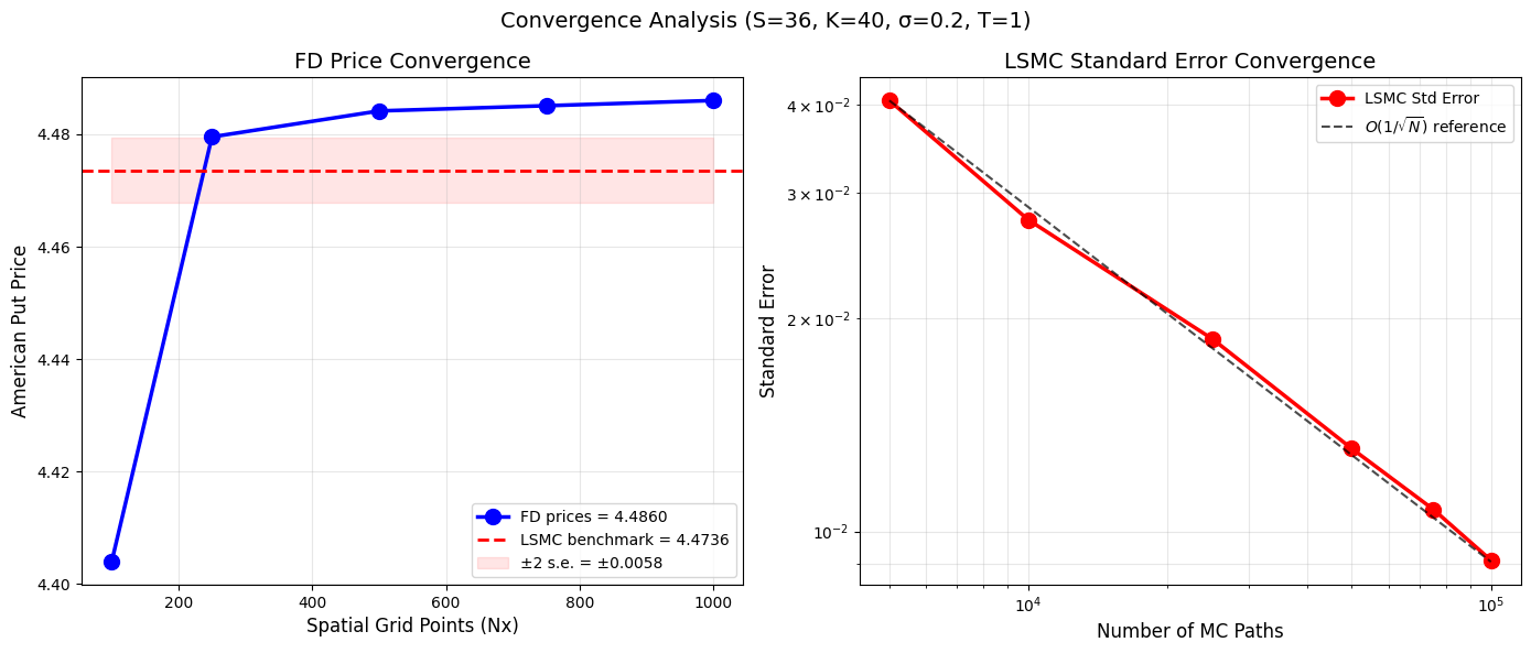
CONVERGENCE SUMMARY
==================================================
FD (Nx=1000, Nt=40000): 4.486006
LSMC benchmark:         4.473597 ± 0.002910
Difference:             0.012409

FD within 2 s.e. of LSMC: False

Question: So, why does it seem that FD is diverging from the MC price?

Noting that {cite:t}LongstaffSchwartz2001 proposes the LSMC method, so we are comparing the LSMC against FD.

• To eliminate any doubts (TODO) implement binomial tree as the reference and compare both LSMC and FD against binomial tree price.

Show code cell source

Hide code cell source

def generate_table1(): # Generates the complete Table 1
    """ Generate complete Table 1 
    Want to show: 
    - Use overkilled LSMC params to get as precise as possible price
    - Does FD-price tend to that value?
        - Plot suggests otherwise
        - In Table there is a slight inaccuracy in AM-price [need to correct]
    """
    # Fixed parameters
    K = 40
    r = 0.06
    
    # Table parameters
    params = [
        (36, 0.20, 1), (36, 0.20, 2), (36, 0.40, 1), (36, 0.40, 2),
        (38, 0.20, 1), (38, 0.20, 2), (38, 0.40, 1), (38, 0.40, 2),
        (40, 0.20, 1), (40, 0.20, 2), (40, 0.40, 1), (40, 0.40, 2),
        (42, 0.20, 1), (42, 0.20, 2), (42, 0.40, 1), (42, 0.40, 2),
        (44, 0.20, 1), (44, 0.20, 2), (44, 0.40, 1), (44, 0.40, 2)
    ]
    
    results = []
    
    for S0, sigma, T in params:
        # Closed form EU
        european = bs_put_price(S0, K, r, sigma, T)
        
        # FD AM put pricer
        american_fd = fd_american_put(S0, K, r, sigma, T)[0]
        early_ex_fd = american_fd - european
        
        # LSMC-pricer
        np.random.seed(1)
        n_steps = int(T * 50)
        S_paths = simulate_gbm_paths(S0, r, sigma, T, n_steps, 50000) # as in paper
        american_lsmc, se_lsmc = lsmc_american_put(S_paths, K, r, T, n_steps)
        early_ex_lsmc = american_lsmc - european
        
        # Difference in early exercise 
        diff = early_ex_lsmc - early_ex_fd
        
        results.append({
            'S': S0, 'sigma': sigma, 'T': T,
            'FD_American': american_fd, 'European': european, 'FD_Early_Ex': early_ex_fd,
            'LSMC_American': american_lsmc, 'SE': se_lsmc, 'LSMC_Early_Ex': early_ex_lsmc,
            'Difference': diff
        })
    
    df = pd.DataFrame(results)
    
    return print(df)

# When we run this is for each triplet in params it computes the LSMC-overkilled which takes too long to compute
#generate_table1()