12. Black-Scholes: From Model to PnL

This notebook covers the complete hedging workflow: pricing an option, computing Greeks, delta-hedging, and decomposing the resulting PnL into its components.

Black-Scholes isn’t really about the formula — it’s about the replicating portfolio. The price is just the cost of setting up the hedge.

Show code cell source

Hide code cell source

import numpy as np
import matplotlib.pyplot as plt
from scipy.stats import norm
import pandas as pd

np.random.seed(42)

12.1. Black-Scholes Pricing and Greeks

The Black-Scholes price for a European call:

\[C(S, t) = S\Phi(d_1) - Ke^{-r\tau}\Phi(d_2)\]

where \(\tau = T - t\) and:

\[d_1 = \frac{\ln(S/K) + (r + \sigma^2/2)\tau}{\sigma\sqrt{\tau}}, \quad d_2 = d_1 - \sigma\sqrt{\tau}\]

The Greeks measure sensitivity to each input. For a call:

• \(\Delta = \Phi(d_1)\)

• \(\Gamma = \phi(d_1)/(S\sigma\sqrt{\tau})\)

• \(\Theta = -S\phi(d_1)\sigma/(2\sqrt{\tau}) - rKe^{-r\tau}\Phi(d_2)\)

• \(\mathcal{V} = S\phi(d_1)\sqrt{\tau}\)

Show code cell source

Hide code cell source

def bs_price(S, K, tau, r, sigma, option_type='call'):
    if tau <= 0:
        if option_type == 'call':
            return max(S - K, 0)
        else:
            return max(K - S, 0)
    
    d1 = (np.log(S / K) + (r + 0.5 * sigma**2) * tau) / (sigma * np.sqrt(tau))
    d2 = d1 - sigma * np.sqrt(tau)
    
    if option_type == 'call':
        return S * norm.cdf(d1) - K * np.exp(-r * tau) * norm.cdf(d2)
    else:
        return K * np.exp(-r * tau) * norm.cdf(-d2) - S * norm.cdf(-d1)


def bs_greeks(S, K, tau, r, sigma, option_type='call'):
    """Compute all Greeks for Black-Scholes."""
    if tau <= 0:
        price = max(S - K, 0) if option_type == 'call' else max(K - S, 0)
        delta = 1.0 if (option_type == 'call' and S > K) else (-1.0 if (option_type == 'put' and S < K) else 0.0)
        return {'price': price, 'delta': delta, 'gamma': 0, 'theta': 0, 'vega': 0, 'rho': 0}
    
    d1 = (np.log(S / K) + (r + 0.5 * sigma**2) * tau) / (sigma * np.sqrt(tau))
    d2 = d1 - sigma * np.sqrt(tau)
    
    phi_d1 = norm.pdf(d1)  # Standard normal PDF
    Phi_d1 = norm.cdf(d1)  # Standard normal CDF
    Phi_d2 = norm.cdf(d2)
    
    # Common calculations
    gamma = phi_d1 / (S * sigma * np.sqrt(tau))
    vega = S * phi_d1 * np.sqrt(tau)
    
    if option_type == 'call':
        price = S * Phi_d1 - K * np.exp(-r * tau) * Phi_d2
        delta = Phi_d1
        theta = -S * phi_d1 * sigma / (2 * np.sqrt(tau)) - r * K * np.exp(-r * tau) * Phi_d2
        rho = K * tau * np.exp(-r * tau) * Phi_d2
    else:
        price = K * np.exp(-r * tau) * norm.cdf(-d2) - S * norm.cdf(-d1)
        delta = -norm.cdf(-d1)
        theta = -S * phi_d1 * sigma / (2 * np.sqrt(tau)) + r * K * np.exp(-r * tau) * norm.cdf(-d2)
        rho = -K * tau * np.exp(-r * tau) * norm.cdf(-d2)
    
    return {
        'price': price,
        'delta': delta,
        'gamma': gamma,
        'theta': theta,
        'vega': vega,
        'rho': rho
    }

Show code cell source

Hide code cell source

# Test the Greeks calculation
S0, K, T, r, sigma = 100, 100, 0.25, 0.05, 0.20

greeks = bs_greeks(S0, K, T, r, sigma, 'call')
print("ATM Call Option Greeks (S=K=100, T=0.25, sigma=20%)")
print("="*50)
for name, value in greeks.items():
    print(f"{name.capitalize():8s}: {value:10.6f}")

ATM Call Option Greeks (S=K=100, T=0.25, sigma=20%)
==================================================
Price   :   4.614997
Delta   :   0.569460
Gamma   :   0.039288
Theta   : -10.474151
Vega    :  19.644000
Rho     :  13.082755

12.2. The Replicating Portfolio

Black-Scholes is fundamentally a statement about replication: a European option can be perfectly replicated by continuously trading \(\Delta_t\) shares of stock and borrowing/lending at the risk-free rate.

The self-financing portfolio \(\Pi_t = \Delta_t S_t + B_t\) satisfies:

\[d\Pi_t = \Delta_t \, dS_t + r B_t \, dt\]

Hedging continuously with the BS delta, the portfolio tracks the option value exactly. We simulate this below to see how well it works in practice.

Show code cell source

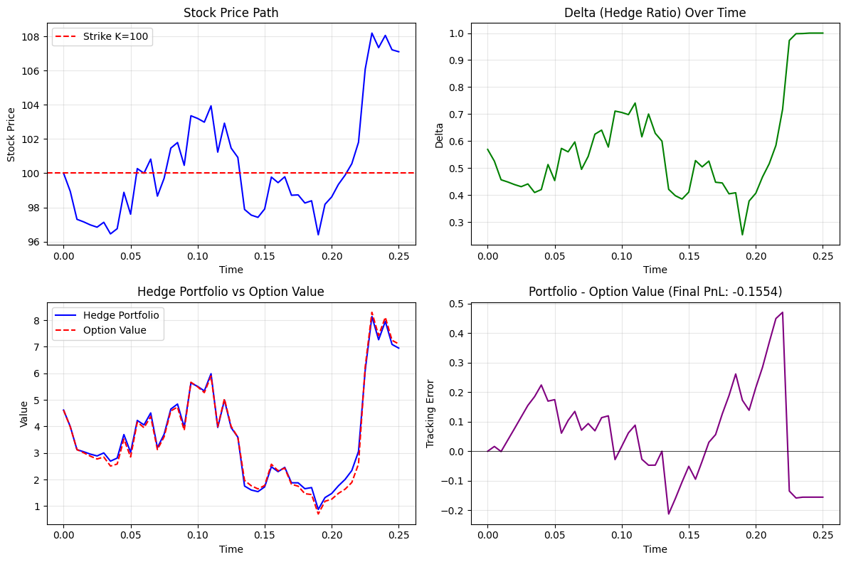
Hide code cell source

def simulate_gbm_path(S0, r, sigma, T, n_steps):
    """Simulate a single GBM path under risk-neutral measure."""
    dt = T / n_steps
    times = np.linspace(0, T, n_steps + 1)
    
    # Generate increments
    dW = np.random.randn(n_steps) * np.sqrt(dt)
    
    # Construct path
    log_returns = (r - 0.5 * sigma**2) * dt + sigma * dW
    prices = S0 * np.exp(np.concatenate([[0], np.cumsum(log_returns)]))
    
    return times, prices

Show code cell source

Hide code cell source

def delta_hedge_simulation(S0, K, T, r, sigma, n_hedge_times, option_type='call'):
    """ Simulate delta-hedging a short option position.
    We sell an option at t=0 and delta-hedge until expiry.
    """
    dt = T / n_hedge_times
    
    # Simulate stock path (use many substeps for accuracy)
    n_substeps = max(1000, n_hedge_times * 10)
    times_fine, prices_fine = simulate_gbm_path(S0, r, sigma, T, n_substeps)
    
    # Extract prices at hedge times
    hedge_indices = np.linspace(0, n_substeps, n_hedge_times + 1, dtype=int)
    times = times_fine[hedge_indices]
    S = prices_fine[hedge_indices]
    
    # Initial option price (what we receive for selling)
    V0 = bs_price(S0, K, T, r, sigma, option_type)
    
    # Initialize hedge portfolio
    # We are SHORT the option, so we receive V0 and must replicate -V
    greeks_0 = bs_greeks(S0, K, T, r, sigma, option_type)
    delta = greeks_0['delta']
    
    # Portfolio: delta shares + cash
    shares = delta
    cash = V0 - delta * S0  # After buying delta shares
    
    # Track everything
    portfolio_values = [V0]
    option_values = [V0]
    deltas = [delta]
    cash_positions = [cash]
    share_positions = [shares]
    
    # Step through time
    for i in range(1, n_hedge_times + 1):
        tau = T - times[i]  # Time remaining
        
        # Cash grows at risk-free rate
        cash *= np.exp(r * dt)
        
        # Current portfolio value (before rebalancing)
        portfolio_value = shares * S[i] + cash
        
        # Current option value
        option_value = bs_price(S[i], K, tau, r, sigma, option_type)
        
        # New delta
        if tau > 0:
            new_greeks = bs_greeks(S[i], K, tau, r, sigma, option_type)
            new_delta = new_greeks['delta']
        else:
            new_delta = 1.0 if (option_type == 'call' and S[i] > K) else 0.0
        
        # Rebalance: buy/sell shares to match new delta
        shares_traded = new_delta - shares
        cash -= shares_traded * S[i]  # Pay for shares
        shares = new_delta
        
        # Store
        portfolio_values.append(portfolio_value)
        option_values.append(option_value)
        deltas.append(new_delta)
        cash_positions.append(cash)
        share_positions.append(shares)
    
    # Final PnL: Portfolio value - Option payoff we must pay
    if option_type == 'call':
        payoff = max(S[-1] - K, 0)
    else:
        payoff = max(K - S[-1], 0)
    
    final_portfolio = shares * S[-1] + cash
    hedge_pnl = final_portfolio - payoff
    
    return {
        'times': times,
        'spot': S,
        'portfolio_values': np.array(portfolio_values),
        'option_values': np.array(option_values),
        'deltas': np.array(deltas),
        'hedge_pnl': hedge_pnl,
        'payoff': payoff,
        'final_portfolio': final_portfolio
    }

Show code cell source

Hide code cell source

# Demonstrate on a single path
S0, K, T, r, sigma = 100, 100, 0.25, 0.05, 0.20

result = delta_hedge_simulation(S0, K, T, r, sigma, n_hedge_times=50, option_type='call')

fig, axes = plt.subplots(2, 2, figsize=(12, 8))

# Stock price path
axes[0, 0].plot(result['times'], result['spot'], 'b-', linewidth=1.5)
axes[0, 0].axhline(K, color='r', linestyle='--', label=f'Strike K={K}')
axes[0, 0].set_xlabel('Time')
axes[0, 0].set_ylabel('Stock Price')
axes[0, 0].set_title('Stock Price Path')
axes[0, 0].legend()
axes[0, 0].grid(True, alpha=0.3)

# Delta over time
axes[0, 1].plot(result['times'], result['deltas'], 'g-', linewidth=1.5)
axes[0, 1].set_xlabel('Time')
axes[0, 1].set_ylabel('Delta')
axes[0, 1].set_title('Delta (Hedge Ratio) Over Time')
axes[0, 1].grid(True, alpha=0.3)

# Portfolio vs Option value
axes[1, 0].plot(result['times'], result['portfolio_values'], 'b-', label='Hedge Portfolio', linewidth=1.5)
axes[1, 0].plot(result['times'], result['option_values'], 'r--', label='Option Value', linewidth=1.5)
axes[1, 0].set_xlabel('Time')
axes[1, 0].set_ylabel('Value')
axes[1, 0].set_title('Hedge Portfolio vs Option Value')
axes[1, 0].legend()
axes[1, 0].grid(True, alpha=0.3)

# Tracking error
tracking_error = result['portfolio_values'] - result['option_values']
axes[1, 1].plot(result['times'], tracking_error, 'purple', linewidth=1.5)
axes[1, 1].axhline(0, color='k', linestyle='-', linewidth=0.5)
axes[1, 1].set_xlabel('Time')
axes[1, 1].set_ylabel('Tracking Error')
axes[1, 1].set_title(f'Portfolio - Option Value (Final PnL: {result["hedge_pnl"]:.4f})')
axes[1, 1].grid(True, alpha=0.3)

plt.tight_layout()
plt.show()

print(f"\nFinal Results:")
print(f"  Option Payoff:     {result['payoff']:.4f}")
print(f"  Portfolio Value:   {result['final_portfolio']:.4f}")
print(f"  Hedge PnL:         {result['hedge_pnl']:.4f}")

Final Results:
  Option Payoff:     7.1043
  Portfolio Value:   6.9489
  Hedge PnL:         -0.1554

12.3. Discrete Hedging and Gamma Bleeding

In practice we can’t hedge continuously—this creates hedging error.

From the Taylor expansion of option value:

\[dV \approx \Delta \, dS + \frac{1}{2}\Gamma (dS)^2 + \Theta \, dt + \mathcal{V} \, d\sigma\]

A delta-hedged portfolio has PnL:

\[d\Pi_{\text{hedged}} = \frac{1}{2}\Gamma (dS)^2 + \Theta \, dt\]

Under continuous hedging, the gamma and theta terms exactly offset (the BS PDE). But with discrete hedging, \((dS)^2 \neq \sigma^2 S^2 dt\) on any given path—realized variance differs from implied. This mismatch creates what traders call “gamma bleeding.”

The standard deviation of discrete hedging PnL scales as \(O(1/\sqrt{n})\) where \(n\) is the number of rebalances.

Show code cell source

Hide code cell source

def analyze_hedge_frequency(S0, K, T, r, sigma, n_paths, hedge_frequencies, option_type='call'):
    """Analyze how hedging frequency affects PnL distribution."""
    results = []
    pnl_distributions = {}
    
    for n_hedge in hedge_frequencies:
        pnls = []
        for _ in range(n_paths):
            sim = delta_hedge_simulation(S0, K, T, r, sigma, n_hedge, option_type)
            pnls.append(sim['hedge_pnl'])
        
        pnls = np.array(pnls)
        pnl_distributions[n_hedge] = pnls
        
        results.append({
            'n_rebalances': n_hedge,
            'mean_pnl': np.mean(pnls),
            'std_pnl': np.std(pnls),
            'min_pnl': np.min(pnls),
            'max_pnl': np.max(pnls),
            '5th_percentile': np.percentile(pnls, 5),
            '95th_percentile': np.percentile(pnls, 95)
        })
    
    return pd.DataFrame(results), pnl_distributions

Show code cell source

Hide code cell source

# Analyze different hedging frequencies
S0, K, T, r, sigma = 100, 100, 0.25, 0.05, 0.20
n_paths = 1000
hedge_frequencies = [5, 10, 25, 50, 100, 250]

print("Running hedge frequency analysis...")
df_freq, pnl_dists = analyze_hedge_frequency(S0, K, T, r, sigma, n_paths, hedge_frequencies)

print("\nHedge Frequency Analysis Results:")
print("="*80)
print(df_freq.to_string(index=False, float_format='{:.6f}'.format))

Running hedge frequency analysis...

Hedge Frequency Analysis Results:
================================================================================
 n_rebalances  mean_pnl  std_pnl   min_pnl  max_pnl  5th_percentile  95th_percentile
            5 -0.027846 1.442597 -5.942480 3.528516       -2.453025         2.265067
           10  0.033356 0.993593 -5.231665 3.047115       -1.609889         1.670701
           25 -0.004569 0.702782 -3.482389 2.371135       -1.141420         1.142473
           50  0.027501 0.491939 -3.283649 1.594189       -0.722729         0.824518
          100  0.013918 0.333773 -1.177576 1.333243       -0.525763         0.586319
          250 -0.005667 0.215202 -0.767826 1.051794       -0.362133         0.336460

Show code cell source

Hide code cell source

fig, axes = plt.subplots(1, 3, figsize=(15, 4))

# PnL Standard Deviation vs Hedge Frequency
axes[0].plot(df_freq['n_rebalances'], df_freq['std_pnl'], 'bo-', linewidth=2, markersize=8)
axes[0].set_xlabel('Number of Rebalances')
axes[0].set_ylabel('PnL Std Dev')
axes[0].set_title('Hedging Error vs Rebalance Frequency')
axes[0].grid(True, alpha=0.3)

# Log-log plot to verify O(1/sqrt(n)) scaling
axes[1].loglog(df_freq['n_rebalances'], df_freq['std_pnl'], 'bo-', linewidth=2, markersize=8)
# Add reference line for 1/sqrt(n) scaling
n_ref = np.array(hedge_frequencies)
scaling = df_freq['std_pnl'].iloc[0] * np.sqrt(hedge_frequencies[0]) / np.sqrt(n_ref)
axes[1].loglog(n_ref, scaling, 'r--', linewidth=2, label=r'$O(1/\sqrt{n})$ scaling')
axes[1].set_xlabel('Number of Rebalances (log)')
axes[1].set_ylabel('PnL Std Dev (log)')
axes[1].set_title('Log-Log Plot: Verifying Scaling Law')
axes[1].legend()
axes[1].grid(True, alpha=0.3)

# PnL Distributions
for n_hedge in [5, 50, 250]:
    axes[2].hist(pnl_dists[n_hedge], bins=50, alpha=0.5, label=f'n={n_hedge}', density=True)
axes[2].axvline(0, color='k', linestyle='--', linewidth=1)
axes[2].set_xlabel('Hedge PnL')
axes[2].set_ylabel('Density')
axes[2].set_title('PnL Distribution by Hedge Frequency')
axes[2].legend()
axes[2].grid(True, alpha=0.3)

plt.tight_layout()
plt.show()

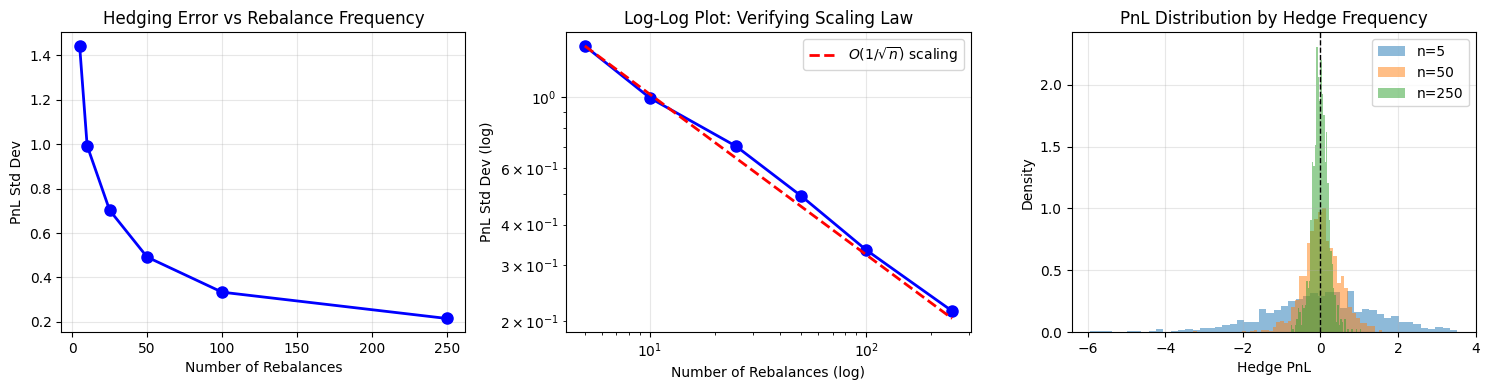
Mean PnL roughly zero, std decreases with hedging frequency. If you think realised vol will exceed implied, you want to be long gamma. Otherwise short gamma.

12.4. PnL Attribution

Every trading desk decomposes daily PnL into Greek components:

\[\Delta\text{PnL} = \underbrace{\Delta \cdot \Delta S}_{\text{delta}} + \underbrace{\frac{1}{2}\Gamma \cdot (\Delta S)^2}_{\text{gamma}} + \underbrace{\Theta \cdot \Delta t}_{\text{theta}} + \underbrace{\mathcal{V} \cdot \Delta\sigma}_{\text{vega}} + \underbrace{\epsilon}_{\text{unexplained}}\]

The unexplained residual is the key diagnostic. If it’s systematically nonzero, your model is missing something. If it’s random noise around zero, your model is capturing the main effects.

Show code cell source

Hide code cell source

def pnl_attribution(V_t, V_t1, greeks_t, S_t, S_t1, sigma_t, sigma_t1, dt):
    actual_pnl = V_t1 - V_t
    dS = S_t1 - S_t
    d_sigma = sigma_t1 - sigma_t
    
    delta_pnl = greeks_t['delta'] * dS
    gamma_pnl = 0.5 * greeks_t['gamma'] * dS**2
    theta_pnl = greeks_t['theta'] * dt
    vega_pnl = greeks_t['vega'] * d_sigma
    
    explained_pnl = delta_pnl + gamma_pnl + theta_pnl + vega_pnl
    unexplained = actual_pnl - explained_pnl
    
    return {
        'actual': actual_pnl,
        'delta': delta_pnl,
        'gamma': gamma_pnl,
        'theta': theta_pnl,
        'vega': vega_pnl,
        'explained': explained_pnl,
        'unexplained': unexplained
    }

Show code cell source

Hide code cell source

def simulate_with_pnl_attribution(S0, K, T, r, sigma, n_steps, option_type='call'):
    """Simulate a path and compute full PnL attribution at each step."""
    dt = T / n_steps
    times, prices = simulate_gbm_path(S0, r, sigma, T, n_steps)
    
    # Store attribution at each step
    attributions = []
    
    for i in range(n_steps):
        tau_t = T - times[i]
        tau_t1 = T - times[i+1]
        
        # Get option values and Greeks
        greeks_t = bs_greeks(prices[i], K, tau_t, r, sigma, option_type)
        V_t = greeks_t['price']
        V_t1 = bs_price(prices[i+1], K, tau_t1, r, sigma, option_type)
        
        # Attribute PnL (constant vol assumption)
        attr = pnl_attribution(V_t, V_t1, greeks_t, prices[i], prices[i+1], sigma, sigma, dt)
        attr['time'] = times[i]
        attr['spot'] = prices[i]
        attributions.append(attr)
    
    return pd.DataFrame(attributions), times, prices

Show code cell source

Hide code cell source

# Run PnL attribution simulation
S0, K, T, r, sigma = 100, 100, 0.25, 0.05, 0.20
n_steps = 63  # Daily for a quarter

attr_df, times, prices = simulate_with_pnl_attribution(S0, K, T, r, sigma, n_steps, 'call')

# Summary statistics
print("PnL Attribution Summary (summed over path):")
print("="*50)
components = ['delta', 'gamma', 'theta', 'vega', 'unexplained', 'actual']
for comp in components:
    total = attr_df[comp].sum()
    print(f"{comp.capitalize():12s}: {total:10.6f}")

print(f"\nExplained %: {100 * attr_df['explained'].sum() / attr_df['actual'].sum():.2f}%")

PnL Attribution Summary (summed over path):
==================================================
Delta       :  -4.630153
Gamma       :   1.072117
Theta       :  -1.078983
Vega        :   0.000000
Unexplained :   0.022022
Actual      :  -4.614997

Explained %: 100.48%

Show code cell source

Hide code cell source

fig, axes = plt.subplots(2, 2, figsize=(14, 10))

# Cumulative PnL by component
ax = axes[0, 0]
for comp, color in [('delta', 'blue'), ('gamma', 'green'), ('theta', 'red'), ('unexplained', 'purple')]:
    ax.plot(attr_df['time'], attr_df[comp].cumsum(), label=comp.capitalize(), linewidth=1.5, color=color)
ax.plot(attr_df['time'], attr_df['actual'].cumsum(), 'k--', label='Actual', linewidth=2)
ax.set_xlabel('Time')
ax.set_ylabel('Cumulative PnL')
ax.set_title('Cumulative PnL Attribution')
ax.legend()
ax.grid(True, alpha=0.3)

# Stacked bar chart of daily attribution
ax = axes[0, 1]
bottom_pos = np.zeros(len(attr_df))
bottom_neg = np.zeros(len(attr_df))
colors = {'delta': 'blue', 'gamma': 'green', 'theta': 'red', 'unexplained': 'purple'}

for comp in ['delta', 'gamma', 'theta', 'unexplained']:
    values = attr_df[comp].values
    pos_vals = np.where(values > 0, values, 0)
    neg_vals = np.where(values < 0, values, 0)
    ax.bar(range(len(attr_df)), pos_vals, bottom=bottom_pos, label=comp.capitalize(), color=colors[comp], alpha=0.7, width=1)
    ax.bar(range(len(attr_df)), neg_vals, bottom=bottom_neg, color=colors[comp], alpha=0.7, width=1)
    bottom_pos += pos_vals
    bottom_neg += neg_vals

ax.axhline(0, color='k', linewidth=0.5)
ax.set_xlabel('Time Step')
ax.set_ylabel('Daily PnL')
ax.set_title('Daily PnL Breakdown')
ax.legend(loc='upper right')
ax.grid(True, alpha=0.3, axis='y')

# Gamma vs Theta relationship
ax = axes[1, 0]
ax.scatter(attr_df['gamma'], -attr_df['theta'], alpha=0.6, s=30)
ax.plot([attr_df['gamma'].min(), attr_df['gamma'].max()], 
        [attr_df['gamma'].min(), attr_df['gamma'].max()], 'r--', label='Perfect offset')
ax.set_xlabel('Gamma PnL')
ax.set_ylabel('-Theta PnL')
ax.set_title('Gamma-Theta Tradeoff (should cluster near line)')
ax.legend()
ax.grid(True, alpha=0.3)

# Unexplained PnL distribution
ax = axes[1, 1]
ax.hist(attr_df['unexplained'], bins=30, edgecolor='black', alpha=0.7)
ax.axvline(0, color='r', linestyle='--', linewidth=2)
ax.axvline(attr_df['unexplained'].mean(), color='g', linestyle='-', linewidth=2, label=f"Mean: {attr_df['unexplained'].mean():.6f}")
ax.set_xlabel('Unexplained PnL')
ax.set_ylabel('Frequency')
ax.set_title('Distribution of Unexplained PnL')
ax.legend()
ax.grid(True, alpha=0.3)

plt.tight_layout()
plt.show()

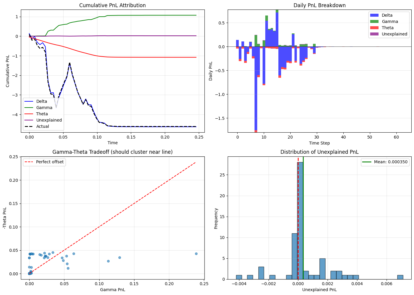
The gamma-theta scatter plot shows the fundamental tradeoff: long gamma means you profit from big moves, but you pay theta every day. Under Black-Scholes with realized vol matching implied, these two effects should cancel out on average.

When they don’t cancel:

• Realized vol > implied vol → gamma PnL exceeds theta cost → long gamma wins

• Realized vol < implied vol → theta cost exceeds gamma PnL → short gamma wins

This is the basis of volatility trading.

12.5. Detecting Model Failure

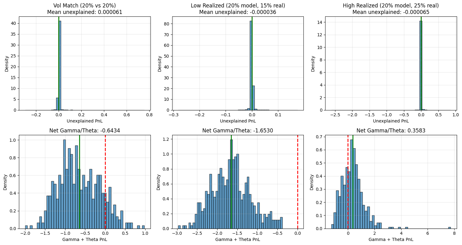
The unexplained PnL should be mean-zero and randomly distributed. When it’s systematically positive or negative, your model is missing something important.

See what happens when we hedge with one volatility but the stock actually moves with a different realized volatility.

Show code cell source

Hide code cell source

def simulate_model_mismatch(S0, K, T, r, sigma_model, sigma_realized, n_steps, n_paths, option_type='call'):
    """ Simulate when realized volatility differs from model volatility.
    - Price and hedge using sigma_model
    - Stock actually moves with sigma_realized
    """
    dt = T / n_steps
    all_unexplained = []
    all_gamma_pnl = []
    all_theta_pnl = []
    hedge_pnls = []
    
    for _ in range(n_paths):
        # Simulate with REALIZED vol
        times, prices = simulate_gbm_path(S0, r, sigma_realized, T, n_steps)
        
        path_unexplained = []
        path_gamma = []
        path_theta = []
        
        for i in range(n_steps):
            tau_t = T - times[i]
            tau_t1 = T - times[i+1]
            
            # Greeks computed with MODEL vol
            greeks_t = bs_greeks(prices[i], K, tau_t, r, sigma_model, option_type)
            
            # Actual option value (priced with model vol, but stock moved with realized vol)
            V_t = greeks_t['price']
            V_t1 = bs_price(prices[i+1], K, tau_t1, r, sigma_model, option_type)
            
            # Attribution
            attr = pnl_attribution(V_t, V_t1, greeks_t, prices[i], prices[i+1], sigma_model, sigma_model, dt)
            path_unexplained.append(attr['unexplained'])
            path_gamma.append(attr['gamma'])
            path_theta.append(attr['theta'])
        
        all_unexplained.extend(path_unexplained)
        all_gamma_pnl.append(sum(path_gamma))
        all_theta_pnl.append(sum(path_theta))
        
        # Total hedge PnL for this path
        hedge_pnls.append(sum(path_gamma) + sum(path_theta))
    
    return {
        'unexplained': np.array(all_unexplained),
        'gamma_pnl': np.array(all_gamma_pnl),
        'theta_pnl': np.array(all_theta_pnl),
        'hedge_pnls': np.array(hedge_pnls)
    }

Show code cell source

Hide code cell source

# Test three scenarios
S0, K, T, r = 100, 100, 0.25, 0.05
sigma_model = 0.20  # What we think vol is (implied vol)
n_steps = 63
n_paths = 500

scenarios = {
    'Vol Match (20% vs 20%)': 0.20,
    'Low Realized (20% model, 15% real)': 0.15,
    'High Realized (20% model, 25% real)': 0.25
}

results = {}
for name, sigma_real in scenarios.items():
    print(f"Running: {name} scenario")
    results[name] = simulate_model_mismatch(S0, K, T, r, sigma_model, sigma_real, n_steps, n_paths)

Running: Vol Match (20% vs 20%) scenario

Running: Low Realized (20% model, 15% real) scenario

Running: High Realized (20% model, 25% real) scenario

Show code cell source

Hide code cell source

fig, axes = plt.subplots(2, 3, figsize=(15, 8))

for idx, (name, data) in enumerate(results.items()):
    # Unexplained distribution
    ax = axes[0, idx]
    ax.hist(data['unexplained'], bins=50, edgecolor='black', alpha=0.7, density=True)
    ax.axvline(0, color='r', linestyle='--', linewidth=2)
    mean_unexp = np.mean(data['unexplained'])
    ax.axvline(mean_unexp, color='g', linestyle='-', linewidth=2)
    ax.set_xlabel('Unexplained PnL')
    ax.set_ylabel('Density')
    ax.set_title(f'{name}\nMean unexplained: {mean_unexp:.6f}')
    ax.grid(True, alpha=0.3)
    
    # Gamma-Theta net
    ax = axes[1, idx]
    net_gamma_theta = data['gamma_pnl'] + data['theta_pnl']
    ax.hist(net_gamma_theta, bins=50, edgecolor='black', alpha=0.7, density=True)
    ax.axvline(0, color='r', linestyle='--', linewidth=2)
    mean_net = np.mean(net_gamma_theta)
    ax.axvline(mean_net, color='g', linestyle='-', linewidth=2)
    ax.set_xlabel('Gamma + Theta PnL')
    ax.set_ylabel('Density')
    ax.set_title(f'Net Gamma/Theta: {mean_net:.4f}')
    ax.grid(True, alpha=0.3)

plt.tight_layout()
plt.show()

print("\nSummary Statistics:")
print("="*70)
for name, data in results.items():
    net = data['gamma_pnl'] + data['theta_pnl']
    print(f"\n{name}:")
    print(f"  Mean Gamma PnL:  {np.mean(data['gamma_pnl']):8.5f}")
    print(f"  Mean Theta PnL:  {np.mean(data['theta_pnl']):8.5f}")
    print(f"  Mean Net:        {np.mean(net):8.5f}")
    print(f"  Std Net:         {np.std(net):8.5f}")

Summary Statistics:
======================================================================

Vol Match (20% vs 20%):
  Mean Gamma PnL:   1.96438
  Mean Theta PnL:  -2.60777
  Mean Net:        -0.64339
  Std Net:          0.51831

Low Realized (20% model, 15% real):
  Mean Gamma PnL:   1.25175
  Mean Theta PnL:  -2.90478
  Mean Net:        -1.65303
  Std Net:          0.48950

High Realized (20% model, 25% real):
  Mean Gamma PnL:   2.81122
  Mean Theta PnL:  -2.45292
  Mean Net:         0.35831
  Std Net:          0.84885

When realised matches implied: gamma/theta PnL nets roughly zero. When they diverge, there’s a systematic edge — short gamma if realised < implied, long gamma if realised > implied. Delta-hedge to isolate the vol bet.

We haven’t modelled transaction costs or execution during vol spikes yet — in practice those eat into returns.

BS survives not because it’s correct but because the hedging framework is robust. Even with non-constant vol, delta-hedging with current implied vol gets you most of the way there. We test this under Heston next.