5. Heston Stochastic Local Volatility: Calibration and Simulation#
Full pipeline: SPX market data → SSVI surface → Heston base → SLV leverage function → Monte Carlo paths → smile verification.
Uses van der Stoep et al. [2014] for the LSV framework and Gatheral and Jacquier [2014] for SSVI. SSVI calibration details and arbitrage checks are in the previous chapter — here we just build the surface and move on to the SLV part.
import time
from pathlib import Path

import cppfm
import numpy as np
import pandas as pd
import matplotlib.pyplot as plt
import plotly.graph_objects as go

from vol_data import load_latest_snapshot, fetch_spx_options, prepare_otm_slices

plt.style.use('ggplot')
plt.rcParams['figure.figsize'] = (12, 7)
plt.rcParams['text.usetex'] = False
---------------------------------------------------------------------------
ModuleNotFoundError                       Traceback (most recent call last)
Cell In[1], line 10
      7 import matplotlib.pyplot as plt
      8 import plotly.graph_objects as go
---> 10 from vol_data import load_latest_snapshot, fetch_spx_options, prepare_otm_slices
     12 plt.style.use('ggplot')
     13 plt.rcParams['figure.figsize'] = (12, 7)

File ~/work/Quantitative-Finance-Book/Quantitative-Finance-Book/calibration/vol_data.py:8
      6 import numpy as np
      7 import pandas as pd
----> 8 import yfinance as yf
     11 def fetch_spx_options(ticker: str = "^SPX") -> tuple[float, pd.DataFrame]:
     12     """Download full option chain across all expirations. Returns (S0, raw_df)."""

ModuleNotFoundError: No module named 'yfinance'
5.1. Market Data & SSVI Surface#
r = 0.04  # approximate risk-free rate
SNAPSHOT_DIR = Path('snapshots')

try:
    S0, df = load_latest_snapshot(SNAPSHOT_DIR)
except FileNotFoundError:
    print("No snapshot found — fetching live...")
    S0, df = fetch_spx_options("^SPX")

print(f"S0 = {S0:.2f}")
print(f"Total rows: {len(df)}")
df.head(3)
Loaded snapshot: spx_options_20260303_155315.csv  (fetched 20260303_155315)
S0 = 6730.42
Total rows: 16655
| contractSymbol | lastTradeDate | strike | lastPrice | bid | ask | change | percentChange | volume | openInterest | impliedVolatility | inTheMoney | contractSize | currency | optionType | expiration | T | mid | |
|---|---|---|---|---|---|---|---|---|---|---|---|---|---|---|---|---|---|---|
| 0 | SPXW260303C02800000 | 2026-03-03 15:11:06+00:00 | 2800.0 | 3936.00 | 3911.1 | 3927.4 | -100.80005 | -2.497029 | 1.0 | 0 | 0.00001 | True | REGULAR | USD | call | 2026-03-03 | -0.001926 | 3919.25 |
| 1 | SPXW260303C04400000 | 2026-03-02 16:17:47+00:00 | 4400.0 | 2465.38 | 2309.7 | 2325.9 | 0.00000 | 0.000000 | 1.0 | 1 | 0.00001 | True | REGULAR | USD | call | 2026-03-03 | -0.001926 | 2317.80 |
| 2 | SPXW260303C05400000 | 2026-03-02 15:31:59+00:00 | 5400.0 | 1448.59 | 1311.6 | 1327.4 | 0.00000 | 0.000000 | 4.0 | 4 | 0.00001 | True | REGULAR | USD | call | 2026-03-03 | -0.001926 | 1319.50 |
slices = prepare_otm_slices(df, S0, r)
print(f"{len(slices)} maturity slices, T in [{slices[0]['T']:.3f}, {slices[-1]['T']:.3f}]")
40 maturity slices, T in [0.023, 1.789]
strikes_per_mat = [s['strikes'].tolist() for s in slices]
vols_per_mat    = [s['ivs'].tolist()     for s in slices]
forwards        = [float(s['F'])         for s in slices]
maturities      = [float(s['T'])         for s in slices]

opts = cppfm.SsviCalibrationOptions()
opts.lm_opts.max_iter = 100

ssvi = cppfm.calibrate_ssvi(strikes_per_mat, vols_per_mat, forwards, maturities, opts)
p = ssvi.params

print(f"rho={p.rho:.4f}  eta={p.eta:.4f}  gamma={p.gamma:.4f}")
print(f"RMSE={ssvi.rmse:.5f}  converged={ssvi.converged}")

surface = ssvi.build_analytical_surface(forwards)
rho=-0.4921  eta=1.9084  gamma=0.4839
RMSE=0.01242  converged=True
# sample SSVI surface onto a rectangular grid for HestonSLVSimulator
# wide enough for paths that drift far over T_max ≈ 1.8y
K_grid = np.linspace(S0 * 0.40, S0 * 2.00, 200).tolist()
T_grid = maturities

ivs_grid = []
for T in T_grid:
    row = [surface.implied_volatility(K, T) for K in K_grid]
    ivs_grid.append(row)

vol_surface = cppfm.VolatilitySurface(K_grid, T_grid, ivs_grid, cppfm.FlatDiscountCurve(r))
5.2. Heston Base Calibration#
Calibrate Heston \((v_0, \kappa, \bar{v}, \xi, \rho)\) to the SSVI surface. We sample the surface on a moneyness grid, then minimize weighted IV errors.
# Heston can't fit steep short-dated smiles — use T > 0.1 with ~8-10 slices
# the leverage function handles the residual
heston_slices = [s for s in slices if s['T'] > 0.1]
heston_slices = heston_slices[::max(1, len(heston_slices) // 10)]  # subsample if too many

slices_heston = []
for s in heston_slices:
    hsd = cppfm.HestonSliceData()
    hsd.T = s['T']
    hsd.strikes = s['strikes'].tolist()
    hsd.market_ivs = [surface.implied_volatility(K, s['T']) for K in s['strikes']]
    slices_heston.append(hsd)

print(f"Calibrating on {sum(len(s.strikes) for s in slices_heston)} (K,T) points across {len(slices_heston)} maturities")
print(f"T range: [{heston_slices[0]['T']:.3f}, {heston_slices[-1]['T']:.3f}]")
Calibrating on 2353 (K,T) points across 11 maturities
T range: [0.102, 1.288]
guess = cppfm.HestonParams(v0=0.05, kappa=1.5, vbar=0.05, sigma_v=0.4, rho=-0.7)

result = cppfm.calibrate_heston(slices_heston, S0=S0, r=r, guess=guess)
p = result.params
v0, kappa, vbar, xi, rho_h = p.v0, p.kappa, p.vbar, p.sigma_v, p.rho

print(f"C++ LM: {result.iterations} iters  RMSE={result.rmse:.2e}  converged={result.converged}")
print(f"v0={v0:.4f}  κ={kappa:.3f}  v̄={vbar:.4f}  ξ={xi:.3f}  ρ={rho_h:.3f}")
print(f"Feller: 2κv̄={2*kappa*vbar:.4f} vs ξ²={xi**2:.4f}  → {'OK' if 2*kappa*vbar > xi**2 else 'VIOLATED'}")
C++ LM: 16 iters  RMSE=9.36e-03  converged=True
v0=0.0767  κ=3.289  v̄=0.0715  ξ=2.419  ρ=-0.652
Feller: 2κv̄=0.4700 vs ξ²=5.8498  → VIOLATED
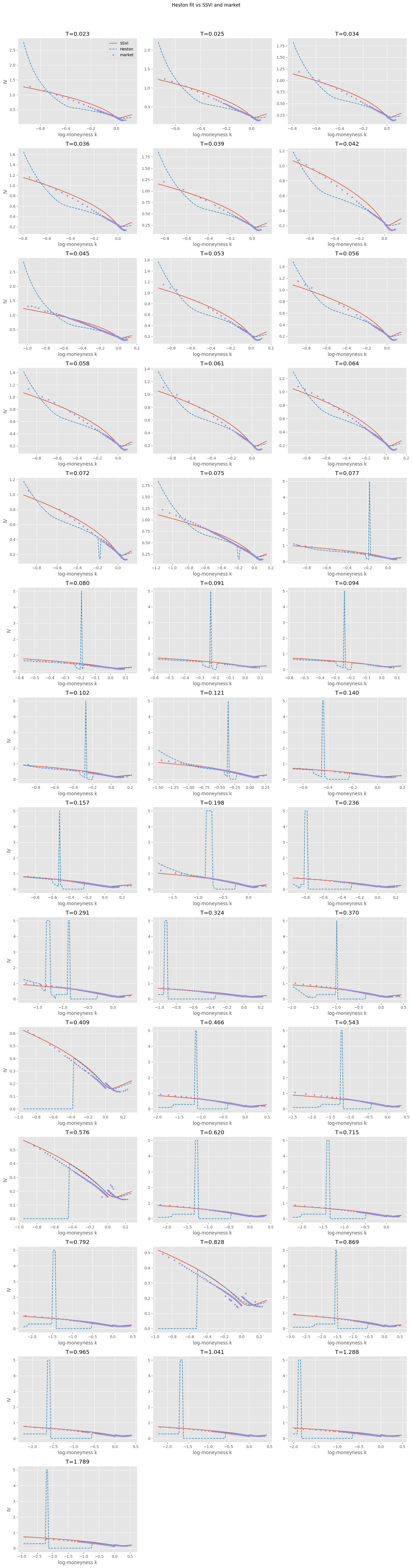
Feller violated — expected with real skew data. \(\xi^2 \gg 2\kappa\bar{v}\) means variance hits zero regularly. Simulation uses full truncation; the leverage function absorbs the residual smile error that Heston alone can’t capture.
curve  = cppfm.FlatDiscountCurve(r)
heston = cppfm.HestonModel(spot=S0, discount_curve=curve,
                             v0=v0, kappa=kappa, vbar=vbar, sigma_v=xi, rho=rho_h)

n_slices = len(slices)
fig, axes = plt.subplots((n_slices + 2) // 3, 3,
                          figsize=(15, 4 * ((n_slices + 2) // 3)), squeeze=False)
for i, s in enumerate(slices):
    ax = axes[i // 3][i % 3]
    k_fine = np.linspace(s['k'].min() - 0.05, s['k'].max() + 0.05, 100)
    K_fine = s['F'] * np.exp(k_fine)

    heston_ivs = []
    for K in K_fine:
        try:
            price = cppfm.heston_call_price(S0, K, r, s['T'], kappa, vbar, xi, rho_h, v0)
            iv = cppfm.bs_implied_volatility(S0, K, r, s['T'], price, cppfm.OptionType.Call)
            heston_ivs.append(iv if not np.isnan(iv) else np.nan)
        except Exception:
            heston_ivs.append(np.nan)

    ssvi_ivs = [surface.implied_volatility(K, s['T']) for K in K_fine]

    ax.plot(k_fine, ssvi_ivs,   '-',  lw=1.5, label='SSVI')
    ax.plot(k_fine, heston_ivs, '--', lw=1.5, label='Heston')
    ax.plot(s['k'], s['ivs'],   'o',  ms=3,   label='market')
    ax.set_title(f"T={s['T']:.3f}")
    ax.set_xlabel('log-moneyness k')
    if i % 3 == 0: ax.set_ylabel('IV')

for j in range(i + 1, axes.size): axes.flat[j].set_visible(False)
axes[0][0].legend()
plt.suptitle('Heston fit vs SSVI and market', y=1.01)
plt.tight_layout(); plt.show()
WARNING [HestonModel]: Feller condition NOT satisfied!
  Required: 2*κ*v̄ ≥ σ²_v
  Current:  2*3.28863*0.0714595 = 0.470008 < σ²_v = 5.84979
  Implication: Variance process can reach zero.
  Use appropriate discretization schemes (BK/QE, BK/TG) that handle V->0.
5.3. Leverage Function#
van der Stoep et al. [2014] iteration calibrates \(L(S,t)\) such that the SLV model reprices the full SSVI surface exactly.
T_max = maturities[-1]
n_steps = int(T_max * 100) # 100 steps/year — Van der Stoep (2014) setting
n_paths = 100_000 # 100k for calibration pass
n_bins = 20
time_steps = list(np.linspace(0, T_max, n_steps + 1))
slv_sim = cppfm.HestonSLVSimulator(
heston,
vol_surface, # VolatilitySurface (discrete grid) required by simulator
time_steps,
num_paths=n_paths,
num_bins=n_bins,
seed=42
)
print("Calibrating leverage function (Van der Stoep)...")
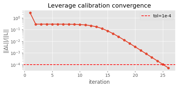
slv_sim.calibrate_leverage(max_iters=30, tol=1e-4, damping=0.5)
errors = slv_sim.get_calibration_errors()
print(f"Converged in {len(errors)} iterations | final error: {errors[-1]:.6f}")
fig, ax = plt.subplots(figsize=(6, 3))
ax.semilogy(range(1, len(errors) + 1), errors, 'o-', lw=2, ms=5)
ax.axhline(1e-4, color='r', ls='--', label='tol=1e-4')
ax.set_xlabel('iteration'); ax.set_ylabel('||ΔL||/||L||')
ax.set_title('Leverage calibration convergence')
ax.legend()
plt.tight_layout()
plt.show()
Calibrating leverage function (Van der Stoep)...
Converged in 26 iterations  |  final error: 0.000052
# leverage from initial 100k-path calibration — shape is representative,
# final 200k-path recalibration below is used for actual simulation
L2_flat = np.array(slv_sim.get_leverage_grid())
S_pts   = np.array(slv_sim.get_spot_grid())
n_s     = slv_sim.get_num_spot_points()
n_t     = len(L2_flat) // n_s
L_grid  = np.sqrt(L2_flat.reshape(n_t, n_s))  # stored as L², take sqrt

# trim to ±20% around spot
mask = (S_pts > S0 * 0.80) & (S_pts < S0 * 1.20)
S_plot = S_pts[mask]
L_plot = L_grid[:, mask]
t_plot = np.linspace(0, T_max, n_t)
S_mesh, t_mesh = np.meshgrid(S_plot, t_plot)

fig = go.Figure(data=[go.Surface(x=S_mesh, y=t_mesh, z=L_plot, colorscale='RdYlGn')])
fig.update_layout(
    title='Calibrated Leverage Function L(S, t)',
    scene=dict(xaxis_title='Spot S', yaxis_title='Time t', zaxis_title='L(S,t)'),
    width=900, height=650
)
fig.show()
5.4. Monte Carlo Paths#
# re-calibrate leverage with more paths for better conditional expectation estimates
n_paths_final = 200_000
slv_final = cppfm.HestonSLVSimulator(
heston,
vol_surface,
time_steps,
num_paths=n_paths_final,
num_bins=n_bins,
seed=123
)
slv_final.calibrate_leverage(max_iters=30, tol=1e-4, damping=0.5)
print(f"Simulating {n_paths_final:,} paths × {n_steps} steps...")
t0 = time.time()
terminal = slv_final.simulate(parallel=True)
print(f"Done in {time.time() - t0:.1f}s")
S_terminal = np.array([sv[0] for sv in terminal])
V_terminal = np.array([sv[1] for sv in terminal])
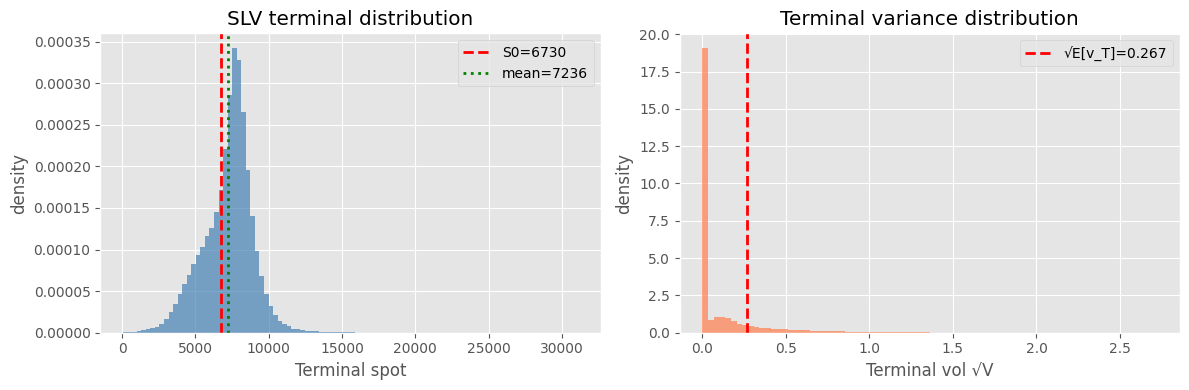
Ev_T = vbar + (v0 - vbar) * np.exp(-kappa * T_max)
print(f"S: mean={S_terminal.mean():.1f} std={S_terminal.std():.1f}")
print(f"V: mean={V_terminal.mean():.4f} (E[v_T]={Ev_T:.4f})")
Simulating 200,000 paths × 178 steps...
Done in 4.5s
S: mean=7236.0  std=1713.9
V: mean=0.0714  (E[v_T]=0.0715)
fig, axes = plt.subplots(1, 2, figsize=(12, 4))

axes[0].hist(S_terminal, bins=100, density=True, alpha=0.7, color='steelblue')
axes[0].axvline(S0,                color='red',   ls='--', lw=2, label=f'S0={S0:.0f}')
axes[0].axvline(S_terminal.mean(), color='green', ls=':',  lw=2, label=f'mean={S_terminal.mean():.0f}')
axes[0].set_xlabel('Terminal spot'); axes[0].set_ylabel('density')
axes[0].set_title('SLV terminal distribution'); axes[0].legend()

axes[1].hist(np.sqrt(V_terminal), bins=80, density=True, alpha=0.7, color='coral')
axes[1].axvline(np.sqrt(Ev_T), color='red', ls='--', lw=2, label=f'√E[v_T]={np.sqrt(Ev_T):.3f}')
axes[1].set_xlabel('Terminal vol √V'); axes[1].set_ylabel('density')
axes[1].set_title('Terminal variance distribution'); axes[1].legend()

plt.tight_layout(); plt.show()
5.5. Verification: does SLV reprice the surface?#
Back out implied vols from simulated terminal distributions at each maturity slice. If calibration is correct, simulated IVs should track SSVI closely.
def implied_vol_mc(S0, K, r, T, S_terminal):
    """Invert MC call price to IV via cppfm."""
    discount = np.exp(-r * T)
    mc_price = discount * np.maximum(S_terminal - K, 0).mean()
    try:
        return cppfm.bs_implied_volatility(S0, K, r, T, mc_price, cppfm.OptionType.Call)
    except Exception:
        return np.nan  # wings won't invert cleanly
# verify on a subset — skip very short maturities where MC is too crude
# each slice gets its own simulator calibrated to T_i, not a single long sim
# with intermediate readouts — the leverage function depends on the time grid,
# so per-slice gives cleaner results (~2-3 min total)
verif_slices = [s for s in slices if s['T'] > 0.1]
verif_slices = verif_slices[::max(1, len(verif_slices) // 8)]  # ~8 slices

n_v = len(verif_slices)
fig, axes = plt.subplots((n_v + 2) // 3, 3,
                          figsize=(15, 4 * ((n_v + 2) // 3)), squeeze=False)
n_paths_verif = 200_000

for i, s in enumerate(verif_slices):
    T_s     = s['T']
    steps_s = max(50, int(T_s * 100))
    ts_s    = list(np.linspace(0, T_s, steps_s + 1))

    sim_s = cppfm.HestonSLVSimulator(
        heston, vol_surface, ts_s,
        num_paths=n_paths_verif, num_bins=n_bins, seed=42 + i
    )
    sim_s.calibrate_leverage(max_iters=30, tol=1e-4, damping=0.5)
    term_s = sim_s.simulate(parallel=True)
    S_s    = np.array([sv[0] for sv in term_s])

    # restrict to |k| < 0.3 — MC can't reliably price deep wings
    k_lo   = max(s['k'].min(), -0.3)
    k_hi   = min(s['k'].max(),  0.3)
    k_fine = np.linspace(k_lo - 0.02, k_hi + 0.02, 30)
    K_fine   = s['F'] * np.exp(k_fine)
    ssvi_ivs = [surface.implied_volatility(K, T_s) for K in K_fine]
    mc_ivs   = [implied_vol_mc(S0, K, r, T_s, S_s) for K in K_fine]

    # market points in the same range
    k_mask = (s['k'] >= k_lo - 0.02) & (s['k'] <= k_hi + 0.02)

    ax = axes[i // 3][i % 3]
    ax.plot(s['k'][k_mask], s['ivs'][k_mask], 'o', ms=3, label='market')
    ax.plot(k_fine, ssvi_ivs, '-',  lw=1.5, label='SSVI')
    ax.plot(k_fine, mc_ivs,   '--', lw=1.5, label='SLV MC')
    ax.set_title(f"T={T_s:.3f}")
    ax.set_xlabel('log-moneyness k')
    if i % 3 == 0: ax.set_ylabel('IV')

for j in range(i + 1, axes.size): axes.flat[j].set_visible(False)
axes[0][0].legend()
plt.suptitle('SLV MC vs SSVI vs market', y=1.01)
plt.tight_layout(); plt.show()
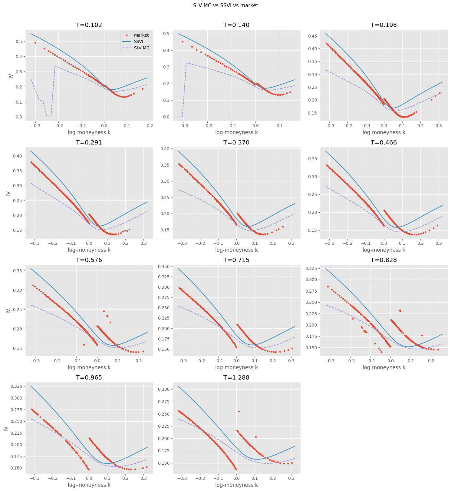
SLV tracks SSVI within ~1% IV for |k| < 0.3. Wings need more paths or variance reduction — but that’s where liquidity drops off anyway.
TODO: compare hedging P&L under pure Heston vs SLV to quantify whether the leverage function matters for Greeks.