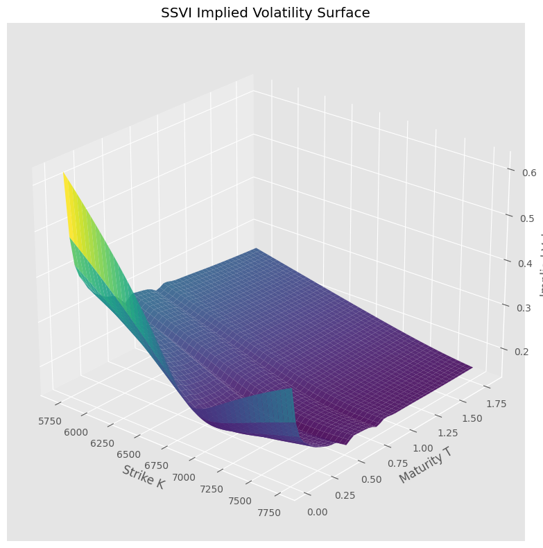
4. SSVI Implied Volatility Surface#
SSVI (Gatheral and Jacquier [2014]) parametrizes total implied variance across the surface with 3 global parameters \((\rho, \eta, \gamma)\) and per-maturity ATM variance \(\theta_T\):
where \(\varphi(\theta) = \frac{\eta}{\theta^\gamma(1+\theta)^{1-\gamma}}\) and \(k = \log(K/F)\).
Calibrate on live SPX options via cppfm.
---------------------------------------------------------------------------
ModuleNotFoundError                       Traceback (most recent call last)
Cell In[1], line 7
      4 import matplotlib.pyplot as plt
      5 from pathlib import Path
----> 7 from vol_data import load_latest_snapshot, fetch_spx_options, prepare_otm_slices
      9 plt.style.use('ggplot')
     10 plt.rcParams['figure.figsize'] = (12, 7)

File ~/work/Quantitative-Finance-Book/Quantitative-Finance-Book/calibration/vol_data.py:8
      6 import numpy as np
      7 import pandas as pd
----> 8 import yfinance as yf
     11 def fetch_spx_options(ticker: str = "^SPX") -> tuple[float, pd.DataFrame]:
     12     """Download full option chain across all expirations. Returns (S0, raw_df)."""

ModuleNotFoundError: No module named 'yfinance'
Loaded snapshot: spx_options_20260303_155315.csv  (fetched 20260303_155315)
S0 = 6730.42
Expirations with data: 51
| contractSymbol | lastTradeDate | strike | lastPrice | bid | ask | change | percentChange | volume | openInterest | impliedVolatility | inTheMoney | contractSize | currency | optionType | expiration | T | mid | |
|---|---|---|---|---|---|---|---|---|---|---|---|---|---|---|---|---|---|---|
| 0 | SPXW260303C02800000 | 2026-03-03 15:11:06+00:00 | 2800.0 | 3936.00 | 3911.1 | 3927.4 | -100.80005 | -2.497029 | 1.0 | 0 | 0.00001 | True | REGULAR | USD | call | 2026-03-03 | -0.001926 | 3919.25 |
| 1 | SPXW260303C04400000 | 2026-03-02 16:17:47+00:00 | 4400.0 | 2465.38 | 2309.7 | 2325.9 | 0.00000 | 0.000000 | 1.0 | 1 | 0.00001 | True | REGULAR | USD | call | 2026-03-03 | -0.001926 | 2317.80 |
| 2 | SPXW260303C05400000 | 2026-03-02 15:31:59+00:00 | 5400.0 | 1448.59 | 1311.6 | 1327.4 | 0.00000 | 0.000000 | 4.0 | 4 | 0.00001 | True | REGULAR | USD | call | 2026-03-03 | -0.001926 | 1319.50 |
| 3 | SPXW260303C05500000 | 2026-03-03 04:38:47+00:00 | 5500.0 | 1329.14 | 1209.7 | 1224.4 | -30.27002 | -2.226703 | 1.0 | 22 | 0.00001 | True | REGULAR | USD | call | 2026-03-03 | -0.001926 | 1217.05 |
| 4 | SPXW260303C05800000 | 2026-03-02 19:49:39+00:00 | 5800.0 | 1097.92 | 912.3 | 927.7 | 0.00000 | 0.000000 | 3.0 | 3 | 0.00001 | True | REGULAR | USD | call | 2026-03-03 | -0.001926 | 920.00 |
40 maturity slices after filtering
| T | F | n_strikes | K_range | k_range | |
|---|---|---|---|---|---|
| 0 | 0.022714 | 6736.5 | 136 | [3400, 7250] | [-0.684, 0.073] |
| 1 | 0.025452 | 6737.3 | 206 | [3400, 7210] | [-0.684, 0.068] |
| 2 | 0.033666 | 6739.5 | 133 | [3200, 7250] | [-0.745, 0.073] |
| 3 | 0.036404 | 6740.2 | 118 | [3200, 7200] | [-0.745, 0.066] |
| 4 | 0.039142 | 6741.0 | 112 | [3000, 7325] | [-0.810, 0.083] |
| 5 | 0.041879 | 6741.7 | 104 | [3400, 7350] | [-0.685, 0.086] |
| 6 | 0.044617 | 6742.4 | 379 | [2500, 7410] | [-0.992, 0.094] |
| 7 | 0.052831 | 6744.7 | 107 | [2800, 7500] | [-0.879, 0.106] |
| 8 | 0.055569 | 6745.4 | 91 | [2800, 7400] | [-0.879, 0.093] |
| 9 | 0.058306 | 6746.1 | 87 | [2800, 7350] | [-0.879, 0.086] |
| 10 | 0.061044 | 6746.9 | 82 | [2800, 7425] | [-0.879, 0.096] |
| 11 | 0.063782 | 6747.6 | 183 | [2800, 7450] | [-0.880, 0.099] |
| 12 | 0.071996 | 6749.8 | 81 | [2800, 7350] | [-0.880, 0.085] |
| 13 | 0.074734 | 6750.6 | 446 | [2200, 7445] | [-1.121, 0.098] |
| 14 | 0.077471 | 6751.3 | 73 | [2800, 7325] | [-0.880, 0.082] |
| 15 | 0.080209 | 6752.0 | 107 | [4000, 7400] | [-0.524, 0.092] |
| 16 | 0.091161 | 6755.0 | 38 | [4000, 7400] | [-0.524, 0.091] |
| 17 | 0.093899 | 6755.7 | 22 | [4000, 7300] | [-0.524, 0.077] |
| 18 | 0.102112 | 6758.0 | 100 | [2800, 8000] | [-0.881, 0.169] |
| 19 | 0.121277 | 6763.1 | 392 | [1600, 8400] | [-1.441, 0.217] |
| 20 | 0.140442 | 6768.3 | 88 | [3600, 7800] | [-0.631, 0.142] |
| 21 | 0.156869 | 6772.8 | 350 | [2800, 8800] | [-0.883, 0.262] |
| 22 | 0.197937 | 6783.9 | 368 | [1200, 9200] | [-1.732, 0.305] |
| 23 | 0.236267 | 6794.3 | 198 | [2800, 8400] | [-0.886, 0.212] |
| 24 | 0.291024 | 6809.2 | 301 | [1200, 9400] | [-1.736, 0.322] |
| 25 | 0.323878 | 6818.2 | 279 | [2600, 8500] | [-0.964, 0.220] |
| 26 | 0.370421 | 6830.9 | 262 | [1000, 10200] | [-1.921, 0.401] |
| 27 | 0.408751 | 6841.4 | 119 | [2800, 8800] | [-0.893, 0.252] |
| 28 | 0.466246 | 6857.1 | 230 | [1000, 10600] | [-1.925, 0.436] |
| 29 | 0.542906 | 6878.2 | 202 | [600, 9400] | [-2.439, 0.312] |
| 30 | 0.575760 | 6887.2 | 269 | [2800, 8600] | [-0.900, 0.222] |
| 31 | 0.619566 | 6899.3 | 182 | [800, 9800] | [-2.155, 0.351] |
| 32 | 0.715391 | 6925.8 | 171 | [800, 9400] | [-2.158, 0.305] |
| 33 | 0.792050 | 6947.1 | 203 | [800, 10600] | [-2.161, 0.423] |
| 34 | 0.827643 | 6957.0 | 218 | [2800, 8800] | [-0.910, 0.235] |
| 35 | 0.868710 | 6968.4 | 188 | [400, 11400] | [-2.858, 0.492] |
| 36 | 0.964535 | 6995.2 | 146 | [800, 10000] | [-2.168, 0.357] |
| 37 | 1.041195 | 7016.6 | 172 | [800, 10200] | [-2.171, 0.374] |
| 38 | 1.287601 | 7086.1 | 200 | [1000, 10800] | [-1.958, 0.421] |
| 39 | 1.788628 | 7229.6 | 132 | [400, 12000] | [-2.894, 0.507] |
4.1. Per-Slice SVI#
SVI fitted independently per maturity — no cross-slice consistency.
| T | a | b | rho | m | sigma | rmse | constraints | converged | |
|---|---|---|---|---|---|---|---|---|---|
| 0 | 0.0227 | -0.007820 | 0.040773 | -0.8649 | -0.1319 | 0.311474 | 0.000126 | False | False |
| 1 | 0.0255 | -0.012185 | 0.046202 | -0.7727 | -0.1231 | 0.371286 | 0.000120 | False | False |
| 2 | 0.0337 | -0.009424 | 0.046188 | -0.9403 | -0.1621 | 0.358919 | 0.000137 | False | True |
| 3 | 0.0364 | -0.012432 | 0.049704 | -0.8528 | -0.1364 | 0.380078 | 0.000136 | False | False |
| 4 | 0.0391 | -0.010864 | 0.049744 | -0.8731 | -0.1288 | 0.349662 | 0.000176 | False | True |
| 5 | 0.0419 | -0.074176 | 0.106509 | -0.1710 | 0.0597 | 0.704510 | 0.000179 | False | False |
| 6 | 0.0446 | -0.020033 | 0.062352 | -0.7090 | -0.1202 | 0.428563 | 0.000317 | False | True |
| 7 | 0.0528 | -0.033368 | 0.077258 | -0.4474 | -0.0365 | 0.480028 | 0.000279 | False | True |
| 8 | 0.0556 | -0.125471 | 0.140830 | -0.0494 | 0.1541 | 0.889251 | 0.000222 | False | False |
| 9 | 0.0583 | -0.147222 | 0.165763 | 0.1126 | 0.2880 | 0.892273 | 0.000215 | False | False |
| 10 | 0.0610 | -0.102609 | 0.149092 | 0.1137 | 0.2427 | 0.694377 | 0.000213 | True | True |
| 11 | 0.0638 | -0.013973 | 0.058995 | -0.8796 | -0.1178 | 0.375390 | 0.000222 | False | True |
| 12 | 0.0720 | -0.048721 | 0.090199 | -0.4697 | -0.0430 | 0.595032 | 0.000169 | False | True |
| 13 | 0.0747 | -0.097255 | 0.133051 | -0.0850 | 0.1340 | 0.733227 | 0.000230 | False | True |
| 14 | 0.0775 | -0.041294 | 0.083819 | -0.5826 | -0.0724 | 0.572630 | 0.000154 | False | True |
| 15 | 0.0802 | -0.086287 | 0.117369 | -0.3070 | 0.0187 | 0.760523 | 0.000165 | False | False |
| 16 | 0.0912 | -0.097491 | 0.126346 | -0.4135 | -0.0839 | 0.832744 | 0.000172 | False | False |
| 17 | 0.0939 | -0.072670 | 0.112320 | -0.2830 | 0.0586 | 0.663290 | 0.000102 | False | False |
| 18 | 0.1021 | -0.188868 | 0.570892 | 0.7277 | 0.6362 | 0.487186 | 0.000273 | True | False |
| 19 | 0.1213 | -0.257239 | 0.451166 | 0.5924 | 0.6707 | 0.712487 | 0.000357 | True | False |
| 20 | 0.1404 | -0.146242 | 0.292218 | 0.4290 | 0.4017 | 0.562989 | 0.000227 | True | False |
| 21 | 0.1569 | -0.174216 | 0.393769 | 0.5550 | 0.4906 | 0.540389 | 0.000281 | True | False |
| 22 | 0.1979 | -0.270646 | 0.397479 | 0.4522 | 0.5464 | 0.773295 | 0.000690 | True | False |
| 23 | 0.2363 | -0.280855 | 0.642331 | 0.6618 | 0.6632 | 0.592476 | 0.000470 | True | False |
| 24 | 0.2910 | -0.192266 | 0.311312 | 0.2778 | 0.3458 | 0.661418 | 0.000630 | True | True |
| 25 | 0.3239 | -0.113139 | 0.205935 | -0.0709 | 0.1250 | 0.581347 | 0.000894 | True | True |
| 26 | 0.3704 | -0.164567 | 0.256804 | 0.0492 | 0.2008 | 0.669908 | 0.000931 | True | True |
| 27 | 0.4088 | -0.086738 | 0.183604 | -0.2845 | 0.0260 | 0.540580 | 0.001508 | True | True |
| 28 | 0.4662 | -0.182032 | 0.265752 | -0.0110 | 0.1770 | 0.720677 | 0.001368 | True | True |
| 29 | 0.5429 | -0.554784 | 0.953005 | 0.6732 | 0.9133 | 0.802775 | 0.001922 | True | False |
| 30 | 0.5758 | 0.009001 | 0.102179 | -0.9990 | -0.1147 | 0.185045 | 0.002913 | True | False |
| 31 | 0.6196 | -0.119212 | 0.216927 | -0.2605 | 0.0421 | 0.633476 | 0.001877 | True | True |
| 32 | 0.7154 | -0.117258 | 0.218050 | -0.3018 | 0.0230 | 0.640767 | 0.002511 | True | True |
| 33 | 0.7921 | -0.093726 | 0.203766 | -0.3990 | -0.0228 | 0.599176 | 0.002829 | True | True |
| 34 | 0.8276 | 0.017274 | 0.112440 | -0.9990 | -0.1278 | 0.171071 | 0.005399 | True | False |
| 35 | 0.8687 | -0.090162 | 0.206647 | -0.4197 | -0.0410 | 0.591396 | 0.003641 | True | True |
| 36 | 0.9645 | -0.041219 | 0.175444 | -0.6499 | -0.1275 | 0.485075 | 0.005041 | True | True |
| 37 | 1.0412 | -0.004106 | 0.151789 | -0.8350 | -0.1596 | 0.353213 | 0.004886 | True | True |
| 38 | 1.2876 | 0.011763 | 0.152370 | -0.8910 | -0.1913 | 0.315645 | 0.007550 | True | True |
| 39 | 1.7886 | -0.015015 | 0.192444 | -0.7079 | -0.1844 | 0.464155 | 0.011758 | True | True |
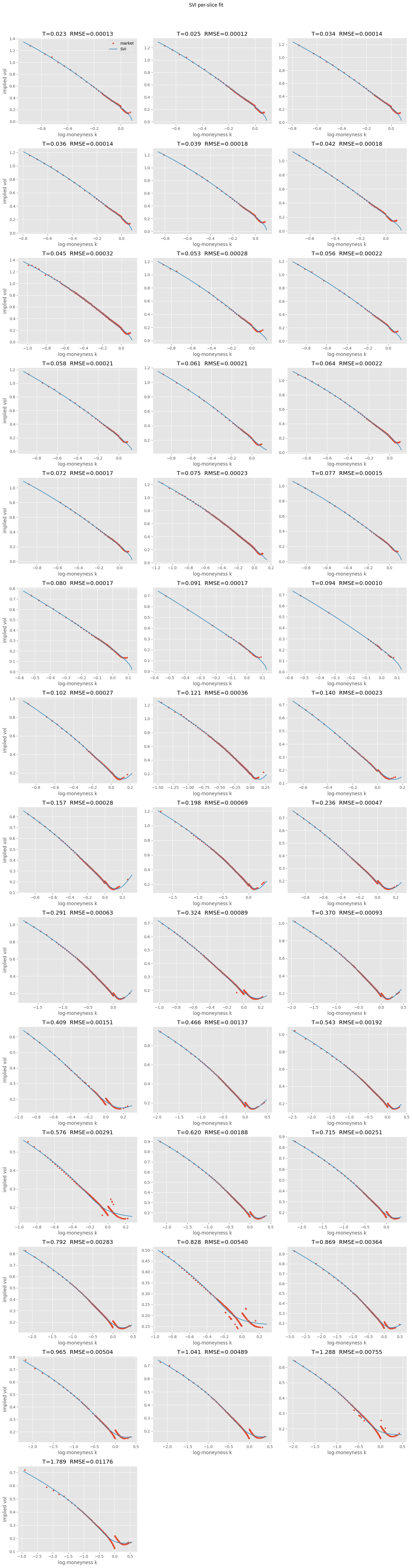
Lots of converged=False on short-dated slices — expected with few strikes and high curvature. Per-slice SVI doesn’t enforce cross-maturity consistency either. SSVI fixes both.
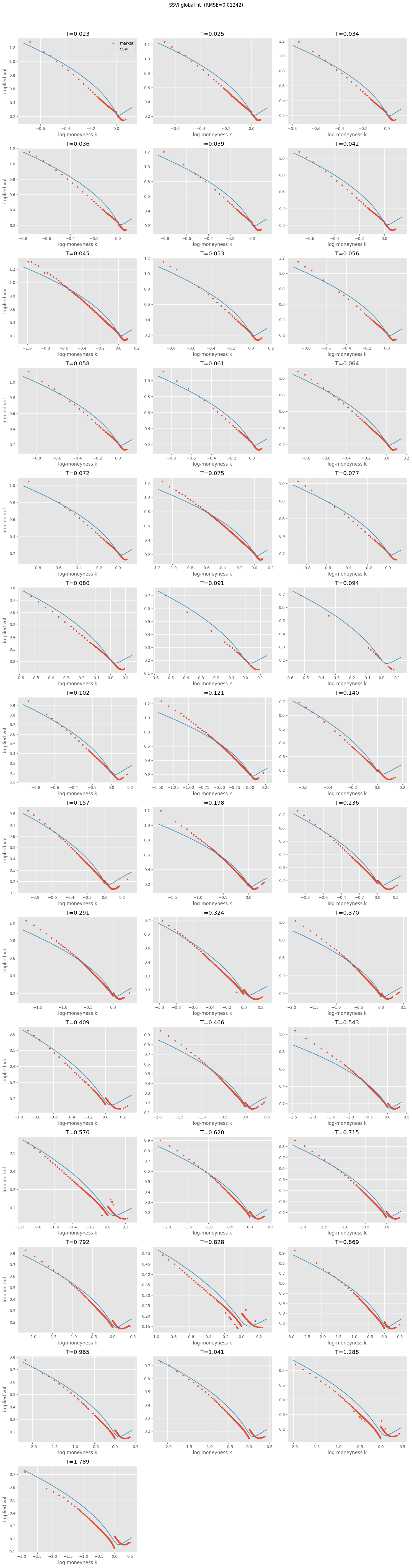
4.2. Global SSVI#
3 global parameters \((\rho, \eta, \gamma)\) + per-maturity \(\theta_T\). Cross-slice consistency enforced.
strikes_per_mat = [s['strikes'].tolist() for s in slices]
vols_per_mat = [s['ivs'].tolist() for s in slices]
forwards = [float(s['F']) for s in slices]
maturities = [float(s['T']) for s in slices]

ssvi_result = cppfm.calibrate_ssvi(strikes_per_mat, vols_per_mat, forwards, maturities)

p = ssvi_result.params
print(f"rho   = {p.rho:.6f}")
print(f"eta   = {p.eta:.6f}")
print(f"gamma = {p.gamma:.6f}")
print(f"RMSE  = {ssvi_result.rmse:.6f}")
print(f"converged     = {ssvi_result.converged}")
print(f"arbitrage_free = {ssvi_result.arbitrage_free}")

# per-maturity thetas
theta_df = pd.DataFrame({
    'T': maturities,
    'theta': ssvi_result.thetas,
    'ATM_vol': [np.sqrt(th / T) for th, T in zip(ssvi_result.thetas, maturities)]
})
theta_df
rho   = -0.492112
eta   = 1.908426
gamma = 0.483876
RMSE  = 0.012420
converged     = True
arbitrage_free = False
| T | theta | ATM_vol | |
|---|---|---|---|
| 0 | 0.022714 | 0.001413 | 0.249402 |
| 1 | 0.025452 | 0.001526 | 0.244895 |
| 2 | 0.033666 | 0.001725 | 0.226365 |
| 3 | 0.036404 | 0.002082 | 0.239138 |
| 4 | 0.039142 | 0.002082 | 0.230624 |
| 5 | 0.041879 | 0.002339 | 0.236326 |
| 6 | 0.044617 | 0.002405 | 0.232151 |
| 7 | 0.052831 | 0.002563 | 0.220268 |
| 8 | 0.055569 | 0.002779 | 0.223629 |
| 9 | 0.058306 | 0.002865 | 0.221651 |
| 10 | 0.061044 | 0.002943 | 0.219557 |
| 11 | 0.063782 | 0.003125 | 0.221362 |
| 12 | 0.071996 | 0.003270 | 0.213117 |
| 13 | 0.074734 | 0.003434 | 0.214344 |
| 14 | 0.077471 | 0.003552 | 0.214133 |
| 15 | 0.080209 | 0.003676 | 0.214094 |
| 16 | 0.091161 | 0.003817 | 0.204616 |
| 17 | 0.093899 | 0.003834 | 0.202071 |
| 18 | 0.102112 | 0.004398 | 0.207537 |
| 19 | 0.121277 | 0.004903 | 0.201069 |
| 20 | 0.140442 | 0.005449 | 0.196966 |
| 21 | 0.156869 | 0.006148 | 0.197963 |
| 22 | 0.197937 | 0.007328 | 0.192409 |
| 23 | 0.236267 | 0.008400 | 0.188552 |
| 24 | 0.291024 | 0.010175 | 0.186988 |
| 25 | 0.323878 | 0.011145 | 0.185498 |
| 26 | 0.370421 | 0.012492 | 0.183639 |
| 27 | 0.408751 | 0.013988 | 0.184989 |
| 28 | 0.466246 | 0.015261 | 0.180916 |
| 29 | 0.542906 | 0.015261 | 0.167658 |
| 30 | 0.575760 | 0.018648 | 0.179970 |
| 31 | 0.619566 | 0.020890 | 0.183620 |
| 32 | 0.715391 | 0.024064 | 0.183407 |
| 33 | 0.792050 | 0.025041 | 0.177808 |
| 34 | 0.827643 | 0.025041 | 0.173943 |
| 35 | 0.868710 | 0.028788 | 0.182042 |
| 36 | 0.964535 | 0.032237 | 0.182817 |
| 37 | 1.041195 | 0.034500 | 0.182030 |
| 38 | 1.287601 | 0.042031 | 0.180673 |
| 39 | 1.788628 | 0.055979 | 0.176911 |
arbitrage_free = False — the sufficient condition \(\eta(1+|\rho|) \leq 2\) from Gatheral and Jacquier [2014] is violated. Sufficient condition though, not necessary — we might still be arbitrage-free. Check numerically below.
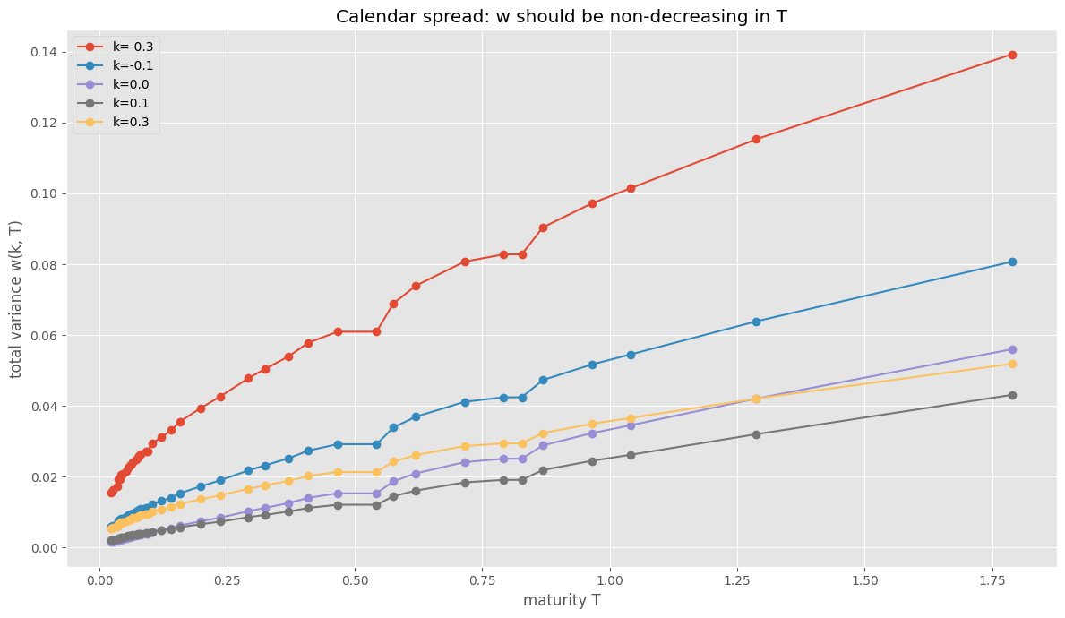
A few theta pairs are flat (monotonicity constraint binding where ATM total variance wanted to decrease).
4.3. Arbitrage checks#
Two conditions for no static arbitrage: butterfly (density \(g(k) \geq 0\)) and calendar spread (total variance non-decreasing in \(T\)).
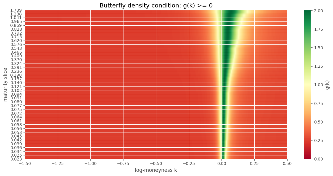
min g(k) across surface: 0.24103993
eta*(1+|rho|) = 2.848  (need <= 2 for Gatheral-Jacquier)
Butterfly failures: 0/40
Calendar failures:  0/40
| T | theta | min_g | butterfly_ok | max_cal_viol | calendar_ok | |
|---|---|---|---|---|---|---|
| 0 | 0.022714 | 0.001413 | 0.248778 | True | 0.0 | True |
| 1 | 0.025452 | 0.001526 | 0.248711 | True | 0.0 | True |
| 2 | 0.033666 | 0.001725 | 0.248600 | True | 0.0 | True |
| 3 | 0.036404 | 0.002082 | 0.248418 | True | 0.0 | True |
| 4 | 0.039142 | 0.002082 | 0.248418 | True | 0.0 | True |
| 5 | 0.041879 | 0.002339 | 0.248299 | True | 0.0 | True |
| 6 | 0.044617 | 0.002405 | 0.248270 | True | 0.0 | True |
| 7 | 0.052831 | 0.002563 | 0.248201 | True | 0.0 | True |
| 8 | 0.055569 | 0.002779 | 0.248112 | True | 0.0 | True |
| 9 | 0.058306 | 0.002865 | 0.248077 | True | 0.0 | True |
| 10 | 0.061044 | 0.002943 | 0.248047 | True | 0.0 | True |
| 11 | 0.063782 | 0.003125 | 0.247977 | True | 0.0 | True |
| 12 | 0.071996 | 0.003270 | 0.247923 | True | 0.0 | True |
| 13 | 0.074734 | 0.003434 | 0.247864 | True | 0.0 | True |
| 14 | 0.077471 | 0.003552 | 0.247822 | True | 0.0 | True |
| 15 | 0.080209 | 0.003676 | 0.247780 | True | 0.0 | True |
| 16 | 0.091161 | 0.003817 | 0.247732 | True | 0.0 | True |
| 17 | 0.093899 | 0.003834 | 0.247726 | True | 0.0 | True |
| 18 | 0.102112 | 0.004398 | 0.247547 | True | 0.0 | True |
| 19 | 0.121277 | 0.004903 | 0.247397 | True | 0.0 | True |
| 20 | 0.140442 | 0.005449 | 0.247246 | True | 0.0 | True |
| 21 | 0.156869 | 0.006148 | 0.247064 | True | 0.0 | True |
| 22 | 0.197937 | 0.007328 | 0.246783 | True | 0.0 | True |
| 23 | 0.236267 | 0.008400 | 0.246550 | True | 0.0 | True |
| 24 | 0.291024 | 0.010175 | 0.246197 | True | 0.0 | True |
| 25 | 0.323878 | 0.011145 | 0.246019 | True | 0.0 | True |
| 26 | 0.370421 | 0.012492 | 0.245784 | True | 0.0 | True |
| 27 | 0.408751 | 0.013988 | 0.245539 | True | 0.0 | True |
| 28 | 0.466246 | 0.015261 | 0.245340 | True | 0.0 | True |
| 29 | 0.542906 | 0.015261 | 0.245340 | True | 0.0 | True |
| 30 | 0.575760 | 0.018648 | 0.244849 | True | 0.0 | True |
| 31 | 0.619566 | 0.020890 | 0.244546 | True | 0.0 | True |
| 32 | 0.715391 | 0.024064 | 0.244142 | True | 0.0 | True |
| 33 | 0.792050 | 0.025041 | 0.244023 | True | 0.0 | True |
| 34 | 0.827643 | 0.025041 | 0.244023 | True | 0.0 | True |
| 35 | 0.868710 | 0.028788 | 0.243581 | True | 0.0 | True |
| 36 | 0.964535 | 0.032237 | 0.243195 | True | 0.0 | True |
| 37 | 1.041195 | 0.034500 | 0.242951 | True | 0.0 | True |
| 38 | 1.287601 | 0.042031 | 0.242184 | True | 0.0 | True |
| 39 | 1.788628 | 0.055979 | 0.241040 | True | 0.0 | True |
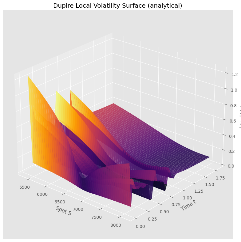
4.4. Implied vol and local vol surfaces#
# analytical Dupire local vol — no grid, no finite differences
S_plot = np.linspace(S0 * 0.8, S0 * 1.2, 100)
T_lv = np.linspace(maturities[0] + 0.01, maturities[-1] - 0.01, 50)
S_mesh, T_lv_mesh = np.meshgrid(S_plot, T_lv)

LV_mesh = np.zeros_like(S_mesh)
for i in range(S_mesh.shape[0]):
    for j in range(S_mesh.shape[1]):
        LV_mesh[i, j] = surface.local_volatility(S_mesh[i, j], T_lv_mesh[i, j])

fig = plt.figure(figsize=(12, 8))
ax = fig.add_subplot(111, projection='3d')
ax.plot_surface(S_mesh, T_lv_mesh, LV_mesh, cmap='inferno', alpha=0.9)
ax.set_xlabel('Spot S')
ax.set_ylabel('Time t')
ax.set_zlabel('Local Vol')
ax.set_title('Dupire Local Volatility Surface (analytical)')
ax.view_init(elev=25, azim=-50)
plt.tight_layout()
plt.show()